SMA BABYVFSSIMP - Treated Before vs After Symptoms
2025-08-11
Read in Data
Read in the data
## Read in data and separate data #############

analysis <- read.csv("~/Library/CloudStorage/Box-Box/CLA RSS Data Sharing/577565_McGrattan_SMA/BABYVFSSIMP/data/SMA_clean_analysis_data_20250811.csv")
chartreview <- read.csv("~/Library/CloudStorage/Box-Box/CLA RSS Data Sharing/577565_McGrattan_SMA/BABYVFSSIMP/data/SMA_clean_chartReview_data_20250811.csv")

#subset the chart review data to only include those in analysis
summary(chartreview$studyid %in% analysis$Subject.ID)

chartreview_foranalysis <- chartreview %>%
  filter(studyid %in% analysis$Subject.ID) %>%
  #and remove the one repeated instance - TX_13; doesn't appear to have any data in that row
  filter(is.na(redcap_repeat_instance))
Included Participants
For this study, include only participants who received treatment:
- sympoms < treatment_age –> Treated after symptoms (had symptoms at younger age than treated) AND symptoms appeared before 6 months
- sympoms > treatment_age –> Treated before symptoms (had symptoms at an older age than treatment) AND have 2 copies of SMN2
- sympoms = “asymptomatic” –> Treated before symptoms
- Had a VFSS before 13 months
chartreview_foranalysis <- chartreview_foranalysis %>%
  rowwise() %>%
  mutate(FirstVisitlessthan13mo = ifelse(age_mbs_1 <= 13, 1, 0),
         Sum_treated = sum(c_across(c(matches("treat_mbs[[:digit:]]___2"), matches("treat_mbs[[:digit:]]___3"), matches("treat_mbs[[:digit:]]___4"), matches("treat_mbs[[:digit:]]___5")))),
         TreatedExam = ifelse(Sum_treated > 0, 1, 0),
         Treated = ifelse(!is.na(treatment_age_c), 1, 0),
         TreatGroup = case_when(is.na(sympoms) ~ "Before Symptoms",
                                sympoms <= treatment_age_c ~ "After Symptoms",
                                sympoms > treatment_age_c ~ "Before Symptoms"),
         SMN2_two = ifelse(smn2c == "2", 1, 0),
         Symptomsbefore6mo = ifelse(sympoms <= 6, 1, 0))

#make sure everyone with a treated exam is included as "treated"
#chartreview_foranalysis$Treated[which(chartreview_foranalysis$TreatedExam==1)]

#override PRI_15 --> should be AFTER SYMPTOMS (double check this)
chartreview_foranalysis$TreatGroup[which(chartreview_foranalysis$studyid == "PRI_15")] <- "After Symptoms"

chartreview_foranalysis %>%
  group_by(FirstVisitlessthan13mo, Treated, TreatedExam, SMN2_two, Symptomsbefore6mo) %>%
  summarize(N = n()) %>%
  ungroup() %>%
  mutate(Percent = N/sum(N)*100) %>%
kable(digits = 2)| FirstVisitlessthan13mo | Treated | TreatedExam | SMN2_two | Symptomsbefore6mo | N | Percent |
|---|---|---|---|---|---|---|
| 0 | 0 | 0 | 0 | 0 | 1 | 0.57 |
| 0 | 1 | 0 | 0 | 1 | 10 | 5.68 |
| 0 | 1 | 1 | 0 | 0 | 1 | 0.57 |
| 0 | 1 | 1 | 0 | 1 | 15 | 8.52 |
| 0 | 1 | 1 | 1 | 0 | 2 | 1.14 |
| 0 | 1 | 1 | 1 | 1 | 21 | 11.93 |
| 0 | 1 | 1 | 1 | NA | 2 | 1.14 |
| 1 | 0 | 0 | 0 | 1 | 14 | 7.95 |
| 1 | 0 | 0 | 1 | 1 | 8 | 4.55 |
| 1 | 1 | 0 | 0 | 1 | 5 | 2.84 |
| 1 | 1 | 0 | 0 | NA | 1 | 0.57 |
| 1 | 1 | 0 | 1 | 0 | 1 | 0.57 |
| 1 | 1 | 0 | 1 | 1 | 11 | 6.25 |
| 1 | 1 | 0 | 1 | NA | 1 | 0.57 |
| 1 | 1 | 1 | 0 | 1 | 7 | 3.98 |
| 1 | 1 | 1 | 0 | NA | 6 | 3.41 |
| 1 | 1 | 1 | 1 | 0 | 1 | 0.57 |
| 1 | 1 | 1 | 1 | 1 | 52 | 29.55 |
| 1 | 1 | 1 | 1 | NA | 17 | 9.66 |
Table of cases to be included:
chartreview_included <- chartreview_foranalysis %>%
  mutate(keep = case_when(TreatGroup == "Before Symptoms" & SMN2_two == 1 ~ 1,
                          TreatGroup == "After Symptoms" & Symptomsbefore6mo == 1 ~ 1,
                          TRUE ~ 0)) %>%
  filter(FirstVisitlessthan13mo == 1, Treated ==1, TreatedExam == 1, keep==1) %>%
  rename(treat_group = TreatGroup)

# chartreview_included %>% select(studyid, treat_group, smn2c, SMN2_two, sympoms, Symptomsbefore6mo, keep) %>% View()

#now take only treated exams where age < 12 months
analysis_included <- analysis %>%
  ungroup() %>%
   mutate(age = as.numeric(age_)) %>%
  #take those in "toinclude" but also only those exams where their age was less than 12 months
  filter(Subject.ID %in% chartreview_included$studyid,
         age <= 13, #updated to 13 to include pp who had exam at 12.032
         treat___1 == 0)

#add treat group to analysis
analysis_included$treat_group <- chartreview_included$treat_group[match(analysis_included$Subject.ID, chartreview_included$studyid)]


chartreview_included %>%
 select(treat_group, treatment_age_c, number_of_mbs, age_mbs_1) %>%
  arrange(treat_group) %>%
kable()| treat_group | treatment_age_c | number_of_mbs | age_mbs_1 |
|---|---|---|---|
| After Symptoms | 5.0000000 | 4 | 7.870000 |
| After Symptoms | 6.6000000 | 3 | 6.570000 |
| After Symptoms | 4.0000000 | 3 | 3.070000 |
| After Symptoms | 6.5700000 | 3 | 7.000000 |
| After Symptoms | 3.0200000 | 2 | 12.880000 |
| After Symptoms | 2.7600000 | 2 | 6.870000 |
| After Symptoms | 2.5300000 | 1 | 7.390000 |
| After Symptoms | 1.0200000 | 1 | 8.210000 |
| After Symptoms | 2.2700000 | 3 | 1.840000 |
| After Symptoms | 0.7600000 | 1 | 4.140000 |
| After Symptoms | 4.5000000 | 1 | 5.300000 |
| After Symptoms | 4.5000000 | 1 | 2.800000 |
| After Symptoms | 4.6000000 | 2 | 2.830000 |
| After Symptoms | 2.1000000 | 4 | 1.610000 |
| After Symptoms | 4.6300000 | 1 | 4.370000 |
| After Symptoms | 4.3000000 | 1 | 8.050000 |
| After Symptoms | 2.3000000 | 1 | 9.990000 |
| After Symptoms | 2.7500000 | 4 | 2.450000 |
| After Symptoms | 8.4400000 | 2 | 8.080000 |
| After Symptoms | 0.8900000 | 3 | 2.230000 |
| After Symptoms | 9.5000000 | 2 | 6.854794 |
| After Symptoms | 3.0200000 | 4 | 4.440000 |
| After Symptoms | 0.4300000 | 3 | 2.960000 |
| After Symptoms | 2.1000000 | 2 | 1.770000 |
| After Symptoms | 8.1100000 | 1 | 7.490000 |
| After Symptoms | 7.4300000 | 3 | 10.020000 |
| After Symptoms | 5.2600000 | 1 | 7.330000 |
| After Symptoms | 10.4500000 | 2 | 7.690000 |
| After Symptoms | 6.7000000 | 3 | 5.950000 |
| After Symptoms | 7.2600000 | 1 | 9.070000 |
| After Symptoms | 7.4300000 | 3 | 5.854794 |
| After Symptoms | 2.0000000 | 1 | 10.800000 |
| After Symptoms | 5.0000000 | 3 | 4.800000 |
| After Symptoms | 9.0300000 | 1 | 11.330000 |
| After Symptoms | 3.0000000 | 2 | 12.450000 |
| After Symptoms | 1.6100000 | 3 | 1.540000 |
| After Symptoms | 0.7200000 | 2 | 0.920000 |
| After Symptoms | 6.1800000 | 1 | 12.880000 |
| After Symptoms | 2.8600000 | 5 | 10.640000 |
| After Symptoms | 13.1400000 | 2 | 12.880000 |
| After Symptoms | 6.6000000 | 5 | 6.540000 |
| After Symptoms | 3.8100000 | 2 | 3.840000 |
| After Symptoms | 2.4600000 | 1 | 7.490000 |
| After Symptoms | 7.2100000 | 2 | 7.640000 |
| After Symptoms | 2.7600000 | 1 | 11.270000 |
| After Symptoms | 1.1200000 | 2 | 1.380000 |
| After Symptoms | 1.1800000 | 1 | 1.220000 |
| After Symptoms | 0.9200000 | 1 | 12.850000 |
| After Symptoms | 0.3900000 | 3 | 2.790000 |
| After Symptoms | 2.5600000 | 4 | 2.370000 |
| After Symptoms | 0.4900000 | 1 | 1.740000 |
| After Symptoms | 0.6900000 | 1 | 1.580000 |
| After Symptoms | 0.6600000 | 3 | 1.250000 |
| After Symptoms | 9.0000000 | 2 | 12.000000 |
| After Symptoms | 4.0000000 | 4 | 4.000000 |
| After Symptoms | 11.0000000 | 2 | 10.000000 |
| After Symptoms | 7.8500000 | 2 | 5.820000 |
| After Symptoms | 2.4300000 | 2 | 1.710000 |
| After Symptoms | 0.7200000 | 1 | 1.640000 |
| Before Symptoms | 0.6600000 | 1 | 3.450000 |
| Before Symptoms | 0.6600000 | 4 | 0.560000 |
| Before Symptoms | 0.3945204 | 4 | 0.000000 |
| Before Symptoms | 0.7600000 | 1 | 6.800000 |
| Before Symptoms | 0.6900000 | 2 | 3.190000 |
| Before Symptoms | 0.0000000 | 3 | 0.000000 |
| Before Symptoms | 0.4600000 | 3 | 0.460000 |
| Before Symptoms | 0.6600000 | 2 | 1.500000 |
| Before Symptoms | 0.0000000 | 5 | 8.674383 |
| Before Symptoms | 0.5000000 | 1 | 6.010000 |
| Before Symptoms | 0.2500000 | 3 | 0.660000 |
| Before Symptoms | 0.0000000 | 1 | 0.560000 |
| Before Symptoms | 0.6904107 | 1 | 0.950000 |
| Before Symptoms | 0.3300000 | 0.260000 | |
| Before Symptoms | 0.8219175 | 1 | 3.000000 |
| Before Symptoms | 0.8547942 | 3 | 7.000000 |
| Before Symptoms | 0.1643835 | 1 | 7.000000 |
# #write out for comparison SMA
# analysis_included %>%
#   select(Subject.ID, studyid_clean, treat_group) %>%
#   arrange(Subject.ID) %>%
#   write.csv(file = "../data/IncludedTreated.csv", row.names = F)

nparts <- length(unique(analysis_included$Subject.ID))

chartreview_included <- chartreview_included %>%
  filter(studyid %in% analysis_included$Subject.ID == T)


# chartreview_included %>%
# select(studyid, treat_group, smn2c, screenc, treatment_age, sympoms_original) %>%
#   arrange(desc(treat_group)) %>%
#   write.csv(file="../data/SMA_InclusionCriteria_TreatBeforeAfter.csv", row.names = F)
Overlap between individuals in this study and Natural history study (prior to treatment)
nathist <- read.csv("~/Library/CloudStorage/Box-Box/CLA RSS Data Sharing/577565_McGrattan_SMA/BABYVFSSIMP/data/SMA_InclusionCriteria_012.csv")

nathist_inc <- nathist %>%
  filter(IncludeDMT == "Yes", IncludeAGE == "Yes")

chartreview_included %>%
  mutate(InNatHist = ifelse(studyid %in% nathist_inc$studyid, "Yes", "No")) %>%
  group_by(InNatHist) %>%
  tally() %>%
  ungroup() %>%
  mutate(percent = n/sum(n)) %>%
kable(digits = 2)| InNatHist | n | percent |
|---|---|---|
| No | 52 | 0.75 |
| Yes | 17 | 0.25 |
Cases not included
Keep only included participants for the reminder of the analysis who have a treated exam and exams where age <= 13 months
chartreview_foranalysis %>%
    filter(studyid %in% chartreview_included$studyid == F) %>%
 select(studyid, TreatGroup, smn2c, sympoms_original, treatment_age_c, age_mbs_1, age_mbs_2, age_mbs_3, age_mbs_4, age_mbs_5) %>%
  arrange(TreatGroup) %>%
  kable()
Create analysis dataset for last exams
analysis_included_lastexam <- analysis_included %>%
  group_by(Subject.ID) %>%
  arrange(desc(visit)) %>%
  slice_head(n=1) %>%
  rowwise() %>%
  mutate(oi_domainI = sum(oi_1, oi_2, oi_3, oi_4, oi_5, oi_6), #scores with NA for oi_4 will be NA for domain_I
         oi_domainII = sum(oi_7, oi_8),
         oi_domainIII = sum(oi_9, oi_10, oi_11, oi_12, oi_13),
         oi_domainIV = sum(oi_14, oi_15),
         oi_domainV = sum(oi_16, oi_17, oi_18, oi_19, oi_20, oi_21))

analysis_included_last_b <- analysis_included_lastexam %>% filter(treat_group == "Before Symptoms")
analysis_included_last_a <- analysis_included_lastexam %>% filter(treat_group == "After Symptoms")
Total Participant Summary
There were a total of 69 participants. Look at participant by number of exams
analysis_included %>%
  group_by(Subject.ID, studyid_clean) %>%
  summarize(count=n()) %>%
  group_by(Subject.ID) %>%
  summarize("N Studies" = n()) %>%
  arrange(desc(`N Studies`)) %>%
  kable()
Treatments
Number of treated vs untreat exams
analysis_included %>%
  group_by(treat_group, Subject.ID) %>%
  summarize(Nexams = n()) %>%
  group_by(treat_group) %>%
  summarize(N_Individuals = n(),
            N_Exams = sum(Nexams)) %>%
kable()| treat_group | N_Individuals | N_Exams |
|---|---|---|
| After Symptoms | 52 | 64 |
| Before Symptoms | 17 | 30 |
Demographics
Sex
chartreview_included %>%
  group_by(sexc) %>%
  summarize(N=n()) %>%
  ungroup() %>%
  mutate(Percent = N/sum(N)*100) %>%
kable(digits = 2)| sexc | N | Percent |
|---|---|---|
| Female | 34 | 49.28 |
| Male | 35 | 50.72 |
chartreview_included %>%
  group_by(sexc, treat_group) %>%
  summarize(N=n()) %>%
  group_by(treat_group) %>%
  mutate(Percent = N/sum(N)*100) %>%
kable(digits = 2)| sexc | treat_group | N | Percent |
|---|---|---|---|
| Female | After Symptoms | 26 | 50.00 |
| Female | Before Symptoms | 8 | 47.06 |
| Male | After Symptoms | 26 | 50.00 |
| Male | Before Symptoms | 9 | 52.94 |
Race: Will recode NA, other, and Unknown/Not Available as Unknown
chartreview_included %>%
  mutate(racec = case_when(racec == "Other" ~ "Unknown",
                           racec == "Unknown/Not Available" ~ "Unknown",
                           is.na(racec) ~ "Unknown",
                           TRUE ~ racec)) %>%
  group_by(racec) %>%
  summarize(N=n()) %>%
  ungroup() %>%
  mutate(Percent = N/sum(N)*100) %>%
kable(digits = 2)| racec | N | Percent |
|---|---|---|
| Asian | 6 | 8.70 |
| Black / African-American | 2 | 2.90 |
| Native American / Alaskan Native | 1 | 1.45 |
| Native Hawaiian / Other Pacific Islander | 1 | 1.45 |
| Unknown | 14 | 20.29 |
| White | 45 | 65.22 |
chartreview_included %>%
  mutate(racec = case_when(racec == "Other" ~ "Unknown",
                           racec == "Unknown/Not Available" ~ "Unknown",
                           is.na(racec) ~ "Unknown",
                           TRUE ~ racec)) %>%
  group_by(racec, treat_group) %>%
  summarize(N=n()) %>%
  group_by(treat_group) %>%
  mutate(Percent = N/sum(N)*100) %>%
kable(digits = 2)| racec | treat_group | N | Percent |
|---|---|---|---|
| Asian | After Symptoms | 5 | 9.62 |
| Asian | Before Symptoms | 1 | 5.88 |
| Black / African-American | After Symptoms | 1 | 1.92 |
| Black / African-American | Before Symptoms | 1 | 5.88 |
| Native American / Alaskan Native | After Symptoms | 1 | 1.92 |
| Native Hawaiian / Other Pacific Islander | After Symptoms | 1 | 1.92 |
| Unknown | After Symptoms | 10 | 19.23 |
| Unknown | Before Symptoms | 4 | 23.53 |
| White | After Symptoms | 34 | 65.38 |
| White | Before Symptoms | 11 | 64.71 |
Number of SMN2 copies
chartreview_included %>%
  group_by(smn2c) %>%
  summarize(N=n()) %>%
  ungroup() %>%
  mutate(Percent = N/sum(N)*100) %>%
kable(digits = 2)| smn2c | N | Percent |
|---|---|---|
| 2 | 65 | 94.2 |
| 3 | 4 | 5.8 |
Number of SMN2 copies by group
chartreview_included %>%
  group_by(smn2c, treat_group) %>%
  summarize(N=n()) %>%
  group_by(treat_group) %>%
  mutate(Percent = N/sum(N)*100) %>%
  arrange(treat_group) %>%
kable(digits = 2)| smn2c | treat_group | N | Percent |
|---|---|---|---|
| 2 | After Symptoms | 48 | 92.31 |
| 3 | After Symptoms | 4 | 7.69 |
| 2 | Before Symptoms | 17 | 100.00 |
Treatment age from chartreview data
chartreview_included %>%
  ungroup() %>%
  summarize(medianTreatmentAge = median(treatment_age_c, na.rm=T),
            IQRTreatmentAge = IQR(treatment_age_c, na.rm=T),
            minTreatmentAge = min(treatment_age_c, na.rm = T),
            maxTreatmentAge = max(treatment_age_c, na.rm = T)) %>%
kable(digits = 2)| medianTreatmentAge | IQRTreatmentAge | minTreatmentAge | maxTreatmentAge |
|---|---|---|---|
| 2.27 | 3.81 | 0 | 11 |
chartreview_included %>%
  group_by(treat_group) %>%
   summarize(medianTreatmentAge = median(treatment_age_c, na.rm=T),
            IQRTreatmentAge = IQR(treatment_age_c, na.rm=T),
            minTreatmentAge = min(treatment_age_c, na.rm=T),
            maxTreatmentAge = max(treatment_age_c, na.rm=T),
            N = n()) %>%
kable(digits = 2)| treat_group | medianTreatmentAge | IQRTreatmentAge | minTreatmentAge | maxTreatmentAge | N |
|---|---|---|---|---|---|
| After Symptoms | 2.81 | 3.56 | 0.39 | 11.00 | 52 |
| Before Symptoms | 0.50 | 0.44 | 0.00 | 0.85 | 17 |
#non-parametric t-test
set.seed(1234)
np.loc.test(x = chartreview_included$treatment_age_c[which(chartreview_included$treat_group == "After Symptoms")],
            y = chartreview_included$treatment_age_c[which(chartreview_included$treat_group == "Before Symptoms")],
            alternative = "two.sided",
            median.test = TRUE,
            paired = FALSE,
            var.equal = FALSE)
Nonparametric Location Test (Studentized Wilcoxon Test)
alternative hypothesis: true median of differences is not equal to 0
t = 17.6781,  p-value = 1e-04
sample estimate:
median of the differences
                  2.36548
cliff.delta(chartreview_included$treatment_age_c[which(chartreview_included$treat_group == "After Symptoms")], chartreview_included$treatment_age_c[which(chartreview_included$treat_group == "Before Symptoms")])
Cliff's Delta

delta estimate: 0.888009 (large)
95 percent confidence interval:
    lower     upper
0.7466309 0.9526383
Specific treatment Note: This is from the pharma_treatment variables, not the treat_mbs ones, as some had only untreated exams so it would indicate no treatment had been given.
chartreview_included <- chartreview_included %>%
  mutate(pharma_treatment___1c = ifelse(pharma_treatment___1 == 1, "None", ""),
         pharma_treatment___2c = ifelse(pharma_treatment___2 == 1, "Nusinersen/Spinraza", ""),
         pharma_treatment___3c = ifelse(pharma_treatment___3 == 1, "AVX-101/Zolgensma", ""),
         pharma_treatment___4c = ifelse(pharma_treatment___4 == 1, "Risdipam", ""),
         pharma_treatment___5c = ifelse(pharma_treatment___5 == 1, "Other", ""))

chartreview_included$treat_combined <- apply(chartreview_included[,c("pharma_treatment___1c", "pharma_treatment___2c", "pharma_treatment___3c", "pharma_treatment___4c", "pharma_treatment___5c")], 1, function(x) paste(x[x != ""], collapse=" & "))

chartreview_included %>%
  mutate(treat_combined = ifelse(grepl("&", treat_combined), "Combination", treat_combined)) %>%
  group_by(treat_combined) %>%
  tally() %>%
  arrange(desc(n)) %>%
  ungroup() %>%
  mutate(percent = n/sum(n)*100) %>%
kable(digits=2)| treat_combined | n | percent |
|---|---|---|
| Combination | 38 | 55.07 |
| Nusinersen/Spinraza | 21 | 30.43 |
| AVX-101/Zolgensma | 7 | 10.14 |
| Risdipam | 3 | 4.35 |
chartreview_included %>%
  mutate(treat_combined = ifelse(grepl("&", treat_combined), "Combination", treat_combined)) %>%
  group_by(treat_combined, treat_group) %>%
  tally() %>%
  arrange(desc(n)) %>%
  group_by(treat_group) %>%
  arrange(treat_group) %>%
  mutate(percent = n/sum(n)*100) %>%
kable(digits=2)| treat_combined | treat_group | n | percent |
|---|---|---|---|
| Combination | After Symptoms | 28 | 53.85 |
| Nusinersen/Spinraza | After Symptoms | 20 | 38.46 |
| AVX-101/Zolgensma | After Symptoms | 3 | 5.77 |
| Risdipam | After Symptoms | 1 | 1.92 |
| Combination | Before Symptoms | 10 | 58.82 |
| AVX-101/Zolgensma | Before Symptoms | 4 | 23.53 |
| Risdipam | Before Symptoms | 2 | 11.76 |
| Nusinersen/Spinraza | Before Symptoms | 1 | 5.88 |
Age at symptom onset - cleaned version Note: symptom onset ages for Lurie_3 and Lurie_7 have been removed, as these were not accurate based on the circumstances the clinicians indicated (both qualified as “overrides” despite recorded age of onset > 6months)
chartreview_included %>%
  ungroup() %>%
 summarize(Median = median(sympoms, na.rm=T),
           Min = min(sympoms, na.rm=T),
           Max = max(sympoms, na.rm=T),
           IQR = IQR(sympoms, na.rm=T),
           N = sum(!is.na(sympoms))) %>%
kable(digits = 2)| Median | Min | Max | IQR | N |
|---|---|---|---|---|
| 1.31 | 0 | 5 | 1.32 | 52 |
chartreview_included %>%
  group_by(treat_group) %>%
 summarize(Median = median(sympoms, na.rm=T),
           Min = min(sympoms, na.rm=T),
           Max = max(sympoms, na.rm=T),
           IQR = IQR(sympoms, na.rm=T),
           N = sum(!is.na(sympoms))) %>%
kable(digits = 2)| treat_group | Median | Min | Max | IQR | N |
|---|---|---|---|---|---|
| After Symptoms | 1.31 | 0 | 5 | 1.32 | 52 |
| Before Symptoms | NA | Inf | -Inf | NA | 0 |
Median age within group
Medians age at last visit
analysis_included_lastexam %>%
  group_by(treat_group) %>%
  summarize(Median_Age = median(age, na.rm=T),
            IQR_Age = IQR(age_, na.rm=T),
            N = n_distinct(Subject.ID),
            N_exams = n()) %>%
kable(digits = 2)| treat_group | Median_Age | IQR_Age | N | N_exams |
|---|---|---|---|---|
| After Symptoms | 8.35 | 4.71 | 52 | 52 |
| Before Symptoms | 6.80 | 5.77 | 17 | 17 |
Are ages last visit different for those who received treatment before vs after symptoms?
set.seed(1234)
np.loc.test(x = analysis_included_last_b$age,
            y = analysis_included_last_a$age,
            alternative = "two.sided",
            median.test = TRUE,
            paired = FALSE,
            var.equal = FALSE)
Nonparametric Location Test (Studentized Wilcoxon Test)
alternative hypothesis: true median of differences is not equal to 0
t = -2.1677,  p-value = 0.0421
sample estimate:
median of the differences
                   -1.915
#effect size using Cliff's Delta - report absolute value of the effect size.
cliff.delta(analysis_included_last_b$age, analysis_included_last_a$age)
Cliff's Delta

delta estimate: -0.3269231 (small)
95 percent confidence interval:
      lower       upper
-0.57988225 -0.01647168
Plot
analysis_included_lastexam %>%
  ggplot(aes(x=treat_group, y=age)) +
  geom_point(position = position_jitter(width = .15)) +
  theme_classic()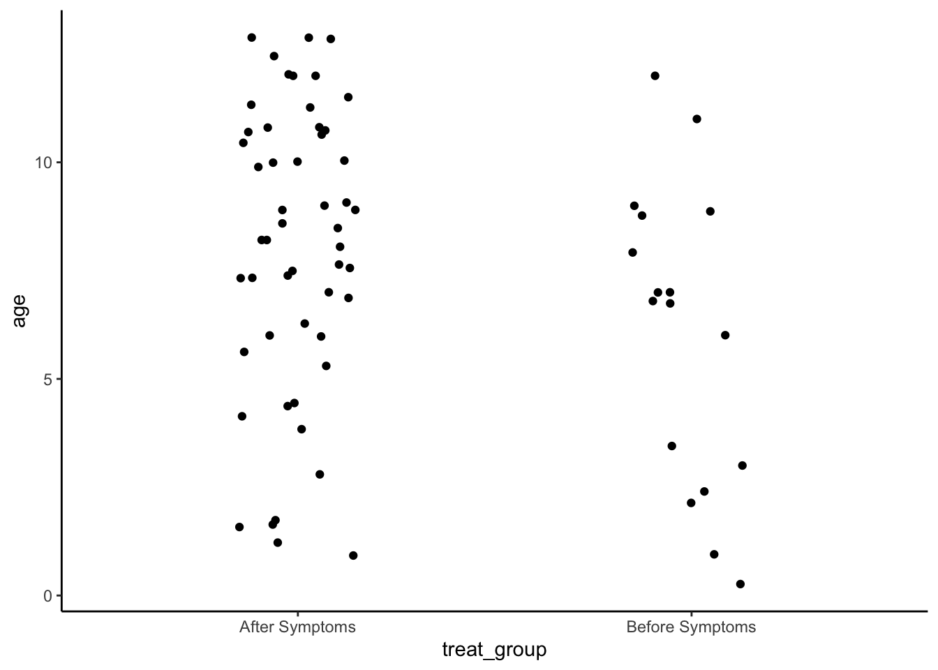
Ethnicity
chartreview_included %>%
  group_by(ethnicityc) %>%
  summarize(N=n()) %>%
  ungroup() %>%
  mutate(Percent = N/sum(N)*100) %>%
kable(digits = 2)| ethnicityc | N | Percent |
|---|---|---|
| Hispanic or Latino | 7 | 10.14 |
| Not Hispanic or Latino | 47 | 68.12 |
| Unknown/Not Available | 14 | 20.29 |
| NA | 1 | 1.45 |
chartreview_included %>%
  mutate(ethnicityc = ifelse(is.na(ethnicityc), "Unknown/Not Available", ethnicityc)) %>%
  group_by(treat_group, ethnicityc) %>%
  summarize(N=n()) %>%
  group_by(treat_group) %>%
  mutate(Percent = N/sum(N)*100) %>%
kable(digits = 2)| treat_group | ethnicityc | N | Percent |
|---|---|---|---|
| After Symptoms | Hispanic or Latino | 6 | 11.54 |
| After Symptoms | Not Hispanic or Latino | 38 | 73.08 |
| After Symptoms | Unknown/Not Available | 8 | 15.38 |
| Before Symptoms | Hispanic or Latino | 1 | 5.88 |
| Before Symptoms | Not Hispanic or Latino | 9 | 52.94 |
| Before Symptoms | Unknown/Not Available | 7 | 41.18 |
Age at initial study
analysis_included %>%
  filter(visit == 1) %>%
  summarize(MedianAge = median(age, na.rm=T),
            IQRAge = IQR(age, na.rm=T),
            MinAge = min(age, na.rm=T),
            MaxAge = max(age, na.rm=T),
            n()) %>%
kable(digits=2)| MedianAge | IQRAge | MinAge | MaxAge | n() |
|---|---|---|---|---|
| 6.01 | 5.93 | 0.26 | 12.88 | 51 |
analysis_included %>%
  filter(visit == 1) %>%
  group_by(treat_group) %>%
  summarize(MedianAge = median(age, na.rm=T),
            IQRAge = IQR(age, na.rm=T),
            MinAge = min(age, na.rm=T),
            MaxAge = max(age, na.rm=T),
            n()) %>%
kable(digits=2)| treat_group | MedianAge | IQRAge | MinAge | MaxAge | n() |
|---|---|---|---|---|---|
| After Symptoms | 7.16 | 7.17 | 0.92 | 12.88 | 38 |
| Before Symptoms | 3.19 | 5.85 | 0.26 | 8.67 | 13 |
#non-parametric t-test
set.seed(1234)
np.loc.test(x = analysis_included$age[which(analysis_included$treat_group == "After Symptoms" & analysis_included$visit == 1)],
            y = analysis_included$age[which(analysis_included$treat_group == "Before Symptoms" & analysis_included$visit == 1)],
            alternative = "two.sided",
            median.test = TRUE,
            paired = FALSE,
            var.equal = FALSE)
Nonparametric Location Test (Studentized Wilcoxon Test)
alternative hypothesis: true median of differences is not equal to 0
t = 2.9041,  p-value = 0.0129
sample estimate:
median of the differences
                 2.647808
cliff.delta(analysis_included$age[which(analysis_included$treat_group == "After Symptoms" & analysis_included$visit == 1)], analysis_included$age[which(analysis_included$treat_group == "Before Symptoms" & analysis_included$visit == 1)])
Cliff's Delta

delta estimate: 0.4534413 (medium)
95 percent confidence interval:
    lower     upper
0.1082704 0.7010443
Other Diagnosis
chartreview_included %>%
  group_by(other_dx) %>%
  summarize(N=n()) %>%
  ungroup() %>%
  mutate(Percent = N/sum(N)*100) %>%
kable(digits = 2)| other_dx | N | Percent |
|---|---|---|
| 44 | 63.77 | |
| Biliary Atresia s/p Kasai, Laryngomalagia s/p supraglottoplasty | 1 | 1.45 |
| FTT | 1 | 1.45 |
| FTT (ongoing following spinraza) | 1 | 1.45 |
| Late preterm 36 weeks | 1 | 1.45 |
| Patient is a preterm infant with medical course complicated by SMA (2 copies SMN2), craniosynostosis s/p posterior cranial vault remodeling and craniotomy with placement of 4 distraction devices (11/14/22) complicated by CVA and seizures, and tongue tie s/p frenotomy (6/14). | 1 | 1.45 |
| Premature 35w 4d | 1 | 1.45 |
| Premature 35w via CS d/t maternal pre-eclampsia | 1 | 1.45 |
| Prematurity 35 6/7 weeks | 1 | 1.45 |
| Prematurity 35w3d | 1 | 1.45 |
| Prematurity 36w | 1 | 1.45 |
| Scoliosis | 1 | 1.45 |
| Tracheomalacia | 1 | 1.45 |
| VFSS at OSH hospital prior to admission which indicated laryngeal penetration and placed the patient on thickened liquids laryngomalacia s/p supraglottoplasty on 6/18/2020; torticollis; G-tube and Nissen fundoplication on 9/23/20 | 1 | 1.45 |
| aspiration PNA with 3 month hospital stay ~ 6 months old | 1 | 1.45 |
| biallelic mutation of SMN1 gene | 1 | 1.45 |
| extralobar sequestration | 1 | 1.45 |
| medistinal mass - normal thymus | 1 | 1.45 |
| milk protein allergy, sleep apnea, plagiocephaly | 1 | 1.45 |
| no | 2 | 2.90 |
| none | 1 | 1.45 |
| paraesophageal hernia | 1 | 1.45 |
| prematurity 35w0d | 1 | 1.45 |
| prematurity 36 w | 1 | 1.45 |
| scoliosis | 1 | 1.45 |
Was genetic testing completed?
chartreview_included %>%
  group_by(genetic_testingc) %>%
  summarize(N=n()) %>%
  ungroup() %>%
  mutate(Percent = N/sum(N)*100) %>%
kable(digits = 2)| genetic_testingc | N | Percent |
|---|---|---|
| Yes | 69 | 100 |
SMA Diagnosed on Newborn Screen?
chartreview_included %>%
  group_by(screenc) %>%
  summarize(N=n()) %>%
  ungroup() %>%
  mutate(Percent = N/sum(N)*100) %>%
kable(digits = 2)| screenc | N | Percent |
|---|---|---|
| No | 42 | 60.87 |
| Yes | 27 | 39.13 |
By group
chartreview_included %>%
  group_by(screenc, treat_group) %>%
  summarize(N=n()) %>%
  ungroup() %>%
  mutate(Percent = N/sum(N)*100) %>%
kable(digits = 2)| screenc | treat_group | N | Percent |
|---|---|---|---|
| No | After Symptoms | 42 | 60.87 |
| Yes | After Symptoms | 10 | 14.49 |
| Yes | Before Symptoms | 17 | 24.64 |
Average number of swallow studies (using the number of exams we have data for)
analysis_included %>%
  group_by(Subject.ID) %>%
  summarize(NumberStudies = n()) %>%
  group_by(NumberStudies) %>%
  summarize(N=n()) %>%
  ungroup() %>%
  mutate(Percent = N/sum(N)*100) %>%
kable(digits = 2)| NumberStudies | N | Percent |
|---|---|---|
| 1 | 52 | 75.36 |
| 2 | 11 | 15.94 |
| 3 | 5 | 7.25 |
| 5 | 1 | 1.45 |
Reason for swallow study referral for last study
analysis_included_lastexam %>%
  group_by(referralc) %>%
  summarize(Nvisits=n()) %>%
  mutate(Percent = Nvisits/sum(Nvisits)*100) %>%
kable(digits = 2)| referralc | Nvisits | Percent |
|---|---|---|
| Asymptomatic, Standard High Risk Referral at Diagnosis | 14 | 20.29 |
| Caregiver reported symptoms | 10 | 14.49 |
| Concerns that swallowing may be contributing to nutritional or respiratory impairments given high risk | 23 | 33.33 |
| Follow-Up from previous impairment | 22 | 31.88 |
analysis_included_lastexam %>%
  group_by(treat_group, referralc) %>%
  summarize(Nvisits=n()) %>%
  group_by(treat_group) %>%
  mutate(Percent = Nvisits/sum(Nvisits)*100) %>%
kable(digits = 2)| treat_group | referralc | Nvisits | Percent |
|---|---|---|---|
| After Symptoms | Asymptomatic, Standard High Risk Referral at Diagnosis | 4 | 7.69 |
| After Symptoms | Caregiver reported symptoms | 9 | 17.31 |
| After Symptoms | Concerns that swallowing may be contributing to nutritional or respiratory impairments given high risk | 17 | 32.69 |
| After Symptoms | Follow-Up from previous impairment | 22 | 42.31 |
| Before Symptoms | Asymptomatic, Standard High Risk Referral at Diagnosis | 10 | 58.82 |
| Before Symptoms | Caregiver reported symptoms | 1 | 5.88 |
| Before Symptoms | Concerns that swallowing may be contributing to nutritional or respiratory impairments given high risk | 6 | 35.29 |
Comparison of “Asymptomatic, Standard High Risk Referral at Diagnosis” values at last exam between groups
analysis_included_lastexam$referralc_asymp = ifelse(analysis_included_lastexam$referralc == "Asymptomatic, Standard High Risk Referral at Diagnosis", "Asymp Visit", "Other")

analysis_included_lastexam %>%
  group_by(treat_group, referralc_asymp) %>%
  tally() %>%
  group_by(treat_group) %>%
  mutate(Percent = n/sum(n)*100) %>%
kable(digits = 2)| treat_group | referralc_asymp | n | Percent |
|---|---|---|---|
| After Symptoms | Asymp Visit | 4 | 7.69 |
| After Symptoms | Other | 48 | 92.31 |
| Before Symptoms | Asymp Visit | 10 | 58.82 |
| Before Symptoms | Other | 7 | 41.18 |
fisher.test(table(analysis_included_lastexam$referralc_asymp, analysis_included_lastexam$treat_group))
    Fisher's Exact Test for Count Data

data:  table(analysis_included_lastexam$referralc_asymp, analysis_included_lastexam$treat_group)
p-value = 3.588e-05
alternative hypothesis: true odds ratio is not equal to 1
95 percent confidence interval:
 0.01094979 0.28393113
sample estimates:
odds ratio
0.06226651
Caregiver symptoms note: check all that apply so possibly multiple symptoms per individual
analysis_included %>%
  select(studyid, visit, caregiver_symptoms1___0:caregiver_symptoms1___8) %>%
  pivot_longer(cols = caregiver_symptoms1___0:caregiver_symptoms1___8,
               names_to = "Symptom",
               values_to = "Selected") %>%
  mutate(Symptomc = case_when(Symptom == "caregiver_symptoms1___0" ~ "Coughing",
                              Symptom == "caregiver_symptoms1___1" ~  "Choking",
                              Symptom == "caregiver_symptoms1___2" ~ "Prolonged Feeding Times",
                              Symptom == "caregiver_symptoms1___3" ~  "Insufficient Volume of Intake",
                              Symptom == "caregiver_symptoms1___4" ~  "Poor Weight Gain",
                              Symptom == "caregiver_symptoms1___5" ~  "Congestion/Wet/Gurgling After Feeds",
                              Symptom == "caregiver_symptoms1___6" ~  "Gagging",
                              Symptom == "caregiver_symptoms1___7" ~  "Spitting out Puree",
                              Symptom == "caregiver_symptoms1___8" ~  "Apnea with feeds")) %>%
  group_by(visit, Symptomc) %>%
  summarize(N = sum(Selected)) %>%
  filter(N != 0) %>%
  group_by(visit) %>%
  mutate(Percent = N/sum(N)*100) %>%
kable(digits = 2)| visit | Symptomc | N | Percent |
|---|---|---|---|
| 1 | Apnea with feeds | 1 | 5.56 |
| 1 | Choking | 3 | 16.67 |
| 1 | Congestion/Wet/Gurgling After Feeds | 4 | 22.22 |
| 1 | Coughing | 5 | 27.78 |
| 1 | Gagging | 2 | 11.11 |
| 1 | Insufficient Volume of Intake | 3 | 16.67 |
| 2 | Coughing | 1 | 100.00 |
Presentations for the last exam - analysis_included arm Note the chart review arm data has 5 options; the analysis_included arm data has 4 options
analysis_included_lastexam %>%
  select(studyid, presentations___1a:presentations___4a) %>%
  pivot_longer(cols = presentations___1a:presentations___4a,
               names_to = "Presentation",
               values_to = "Selected") %>%
  mutate(Presentationc = case_when(Presentation == "presentations___1a" ~ "Thin Liquid",
                              Presentation == "presentations___2a" ~  "Nectar Liquid",
                              Presentation == "presentations___3a" ~ "Honey Liquid",
                              Presentation == "presentations___4a" ~  "Puree")) %>%
  group_by(Presentationc) %>%
 summarize(Count = sum(Selected),
            TotalN = n_distinct(studyid)) %>%
  ungroup() %>%
  mutate(Percent = Count/TotalN*100) %>%
kable(digits = 2)| Presentationc | Count | TotalN | Percent |
|---|---|---|---|
| Honey Liquid | 15 | 69 | 21.74 |
| Nectar Liquid | 30 | 69 | 43.48 |
| Puree | 37 | 69 | 53.62 |
| Thin Liquid | 59 | 69 | 85.51 |
Comparisons for LAST VFSS exam
OI Scores
OI scores between treated before vs after symptoms for last exam
analysis_included_lastexam %>%
  select(Subject.ID, treat_group, matches("oi_[[:digit:]]{1,2}")) %>%
  pivot_longer(cols = starts_with("oi"),
               names_to = "component",
               values_to = "score") %>%
  mutate(component = factor(component, levels = c(paste("oi", 1:21, sep="_")))) %>%
  group_by(component, treat_group) %>%
  summarize(Median_Score = median(score, na.rm=T),
            IQR_Score = IQR(score, na.rm=T),
            Min_Score = min(score, na.rm=T),
            Max_Score = max(score, na.rm = T),
            N_Participants = n(),
            N_Valid_Scores = sum(!is.na(score))) %>%
kable(digits = 2)| component | treat_group | Median_Score | IQR_Score | Min_Score | Max_Score | N_Participants | N_Valid_Scores |
|---|---|---|---|---|---|---|---|
| oi_1 | After Symptoms | 2 | 2 | 0 | 2 | 52 | 52 |
| oi_1 | Before Symptoms | 0 | 1 | 0 | 2 | 17 | 17 |
| oi_2 | After Symptoms | 7 | 2 | 2 | 7 | 52 | 52 |
| oi_2 | Before Symptoms | 6 | 1 | 3 | 7 | 17 | 17 |
| oi_3 | After Symptoms | 2 | 1 | 0 | 2 | 52 | 52 |
| oi_3 | Before Symptoms | 1 | 1 | 0 | 2 | 17 | 17 |
| oi_4 | After Symptoms | 2 | 0 | 2 | 2 | 52 | 52 |
| oi_4 | Before Symptoms | 2 | 0 | 2 | 2 | 17 | 17 |
| oi_5 | After Symptoms | 2 | 0 | 0 | 3 | 52 | 52 |
| oi_5 | Before Symptoms | 2 | 0 | 0 | 2 | 17 | 17 |
| oi_6 | After Symptoms | 2 | 2 | 0 | 2 | 52 | 52 |
| oi_6 | Before Symptoms | 1 | 2 | 0 | 2 | 17 | 17 |
| oi_7 | After Symptoms | 1 | 2 | 0 | 3 | 52 | 52 |
| oi_7 | Before Symptoms | 0 | 0 | 0 | 2 | 17 | 17 |
| oi_8 | After Symptoms | 1 | 2 | 0 | 2 | 52 | 52 |
| oi_8 | Before Symptoms | 0 | 0 | 0 | 2 | 17 | 17 |
| oi_9 | After Symptoms | 2 | 0 | 0 | 3 | 52 | 51 |
| oi_9 | Before Symptoms | 2 | 1 | 0 | 3 | 17 | 17 |
| oi_10 | After Symptoms | 1 | 1 | 0 | 3 | 52 | 51 |
| oi_10 | Before Symptoms | 1 | 1 | 0 | 1 | 17 | 17 |
| oi_11 | After Symptoms | 4 | 2 | 0 | 4 | 52 | 51 |
| oi_11 | Before Symptoms | 2 | 1 | 0 | 4 | 17 | 17 |
| oi_12 | After Symptoms | 2 | 0 | 0 | 2 | 52 | 51 |
| oi_12 | Before Symptoms | 2 | 1 | 0 | 2 | 17 | 17 |
| oi_13 | After Symptoms | 2 | 1 | 0 | 3 | 52 | 51 |
| oi_13 | Before Symptoms | 2 | 1 | 0 | 3 | 17 | 17 |
| oi_14 | After Symptoms | 2 | 2 | 0 | 2 | 52 | 51 |
| oi_14 | Before Symptoms | 0 | 1 | 0 | 2 | 17 | 17 |
| oi_15 | After Symptoms | 2 | 2 | 0 | 3 | 52 | 51 |
| oi_15 | Before Symptoms | 0 | 2 | 0 | 2 | 17 | 17 |
| oi_16 | After Symptoms | 1 | 1 | 0 | 2 | 52 | 52 |
| oi_16 | Before Symptoms | 0 | 1 | 0 | 2 | 17 | 17 |
| oi_17 | After Symptoms | 2 | 1 | 2 | 4 | 52 | 52 |
| oi_17 | Before Symptoms | 2 | 0 | 1 | 2 | 17 | 17 |
| oi_18 | After Symptoms | 1 | 1 | 0 | 2 | 52 | 52 |
| oi_18 | Before Symptoms | 0 | 0 | 0 | 2 | 17 | 17 |
| oi_19 | After Symptoms | 2 | 1 | 1 | 4 | 52 | 52 |
| oi_19 | Before Symptoms | 2 | 1 | 0 | 2 | 17 | 17 |
| oi_20 | After Symptoms | 2 | 1 | 0 | 4 | 52 | 52 |
| oi_20 | Before Symptoms | 1 | 1 | 0 | 2 | 17 | 17 |
| oi_21 | After Symptoms | 1 | 1 | 0 | 3 | 52 | 52 |
| oi_21 | Before Symptoms | 0 | 1 | 0 | 2 | 17 | 17 |
Look at the table of counts and proportions for each score (last exam)
analysis_included_lastexam %>%
  select(Subject.ID, treat_group, matches("oi_[[:digit:]]{1,2}")) %>%
  pivot_longer(cols = starts_with("oi"),
               names_to = "component",
               values_to = "score") %>%
  mutate(component = factor(component, levels = c(paste("oi", 1:21, sep="_")))) %>%
  filter(!is.na(score)) %>%
  group_by(component, treat_group, score) %>%
  summarize(N = n()) %>%
  group_by(component, treat_group) %>%
  mutate(Percent = N/sum(N)*100,
         N_Percent = paste0(N," (", round(Percent,0), "%) ")) %>%
  select(-N, -Percent) %>%
  pivot_wider(names_from = treat_group,
              values_from = N_Percent,
              values_fill = "0 (0%)") %>%
kable(digits = 2)| component | score | After Symptoms | Before Symptoms |
|---|---|---|---|
| oi_1 | 0 | 21 (40%) | 12 (71%) |
| oi_1 | 1 | 3 (6%) | 1 (6%) |
| oi_1 | 2 | 28 (54%) | 4 (24%) |
| oi_2 | 2 | 2 (4%) | 0 (0%) |
| oi_2 | 3 | 2 (4%) | 1 (6%) |
| oi_2 | 4 | 7 (13%) | 2 (12%) |
| oi_2 | 5 | 5 (10%) | 5 (29%) |
| oi_2 | 6 | 7 (13%) | 5 (29%) |
| oi_2 | 7 | 29 (56%) | 4 (24%) |
| oi_3 | 0 | 5 (10%) | 1 (6%) |
| oi_3 | 1 | 20 (38%) | 11 (65%) |
| oi_3 | 2 | 27 (52%) | 5 (29%) |
| oi_4 | 2 | 52 (100%) | 17 (100%) |
| oi_5 | 0 | 1 (2%) | 1 (6%) |
| oi_5 | 2 | 49 (94%) | 16 (94%) |
| oi_5 | 3 | 2 (4%) | 0 (0%) |
| oi_6 | 0 | 15 (29%) | 6 (35%) |
| oi_6 | 1 | 9 (17%) | 5 (29%) |
| oi_6 | 2 | 28 (54%) | 6 (35%) |
| oi_7 | 0 | 23 (44%) | 13 (76%) |
| oi_7 | 1 | 7 (13%) | 3 (18%) |
| oi_7 | 2 | 18 (35%) | 1 (6%) |
| oi_7 | 3 | 4 (8%) | 0 (0%) |
| oi_8 | 0 | 22 (42%) | 13 (76%) |
| oi_8 | 1 | 10 (19%) | 3 (18%) |
| oi_8 | 2 | 20 (38%) | 1 (6%) |
| oi_9 | 0 | 5 (10%) | 1 (6%) |
| oi_9 | 1 | 3 (6%) | 4 (24%) |
| oi_9 | 2 | 36 (71%) | 11 (65%) |
| oi_9 | 3 | 7 (14%) | 1 (6%) |
| oi_10 | 0 | 6 (12%) | 7 (41%) |
| oi_10 | 1 | 22 (43%) | 10 (59%) |
| oi_10 | 2 | 21 (41%) | 0 (0%) |
| oi_10 | 3 | 2 (4%) | 0 (0%) |
| oi_11 | 0 | 4 (8%) | 1 (6%) |
| oi_11 | 1 | 2 (4%) | 1 (6%) |
| oi_11 | 2 | 11 (22%) | 10 (59%) |
| oi_11 | 4 | 34 (67%) | 4 (24%) |
| oi_11 | 3 | 0 (0%) | 1 (6%) |
| oi_12 | 0 | 4 (8%) | 1 (6%) |
| oi_12 | 1 | 4 (8%) | 4 (24%) |
| oi_12 | 2 | 43 (84%) | 12 (71%) |
| oi_13 | 0 | 4 (8%) | 1 (6%) |
| oi_13 | 1 | 4 (8%) | 2 (12%) |
| oi_13 | 2 | 28 (55%) | 9 (53%) |
| oi_13 | 3 | 15 (29%) | 5 (29%) |
| oi_14 | 0 | 15 (29%) | 11 (65%) |
| oi_14 | 1 | 8 (16%) | 4 (24%) |
| oi_14 | 2 | 28 (55%) | 2 (12%) |
| oi_15 | 0 | 15 (29%) | 11 (65%) |
| oi_15 | 1 | 10 (20%) | 1 (6%) |
| oi_15 | 2 | 25 (49%) | 5 (29%) |
| oi_15 | 3 | 1 (2%) | 0 (0%) |
| oi_16 | 0 | 10 (19%) | 10 (59%) |
| oi_16 | 1 | 18 (35%) | 6 (35%) |
| oi_16 | 2 | 24 (46%) | 1 (6%) |
| oi_17 | 2 | 32 (62%) | 16 (94%) |
| oi_17 | 3 | 18 (35%) | 0 (0%) |
| oi_17 | 4 | 2 (4%) | 0 (0%) |
| oi_17 | 1 | 0 (0%) | 1 (6%) |
| oi_18 | 0 | 14 (27%) | 13 (76%) |
| oi_18 | 1 | 28 (54%) | 3 (18%) |
| oi_18 | 2 | 10 (19%) | 1 (6%) |
| oi_19 | 1 | 6 (12%) | 5 (29%) |
| oi_19 | 2 | 28 (54%) | 11 (65%) |
| oi_19 | 3 | 9 (17%) | 0 (0%) |
| oi_19 | 4 | 9 (17%) | 0 (0%) |
| oi_19 | 0 | 0 (0%) | 1 (6%) |
| oi_20 | 0 | 2 (4%) | 3 (18%) |
| oi_20 | 1 | 8 (15%) | 6 (35%) |
| oi_20 | 2 | 25 (48%) | 8 (47%) |
| oi_20 | 3 | 8 (15%) | 0 (0%) |
| oi_20 | 4 | 9 (17%) | 0 (0%) |
| oi_21 | 0 | 12 (23%) | 10 (59%) |
| oi_21 | 1 | 21 (40%) | 6 (35%) |
| oi_21 | 2 | 10 (19%) | 1 (6%) |
| oi_21 | 3 | 9 (17%) | 0 (0%) |
What are the domain scores for last exam?
Sum OI scores across components within domains
- Domain I - components 1,2,3 4, 5, 6
- Domain II - components 7, 8
- Domain III - 9, 10, 11, 12, 13
- Domain IV - 14, 15
- Domain V - 16, 17, 18, 19, 20, 21
Average composite scores overall
analysis_included_lastexam %>%
  select(Subject.ID, treat_group, starts_with("oi_domain")) %>%
  pivot_longer(cols = starts_with("oi_domain"),
               names_to = "domain",
               values_to = "score") %>%
  group_by(domain, treat_group) %>%
  summarize(Median_Score = median(score, na.rm=T),
            IQR_Score = IQR(score, na.rm=T),
            Min_Score = min(score, na.rm=T),
            Max_Score = max(score, na.rm = T),
            N_Participants = n(),
            N_Valid_Scores = sum(!is.na(score))) %>%
kable(digits = 2)| domain | treat_group | Median_Score | IQR_Score | Min_Score | Max_Score | N_Participants | N_Valid_Scores |
|---|---|---|---|---|---|---|---|
| oi_domainI | After Symptoms | 15 | 6.00 | 5 | 18 | 52 | 52 |
| oi_domainI | Before Symptoms | 12 | 3.00 | 8 | 17 | 17 | 17 |
| oi_domainII | After Symptoms | 2 | 4.00 | 0 | 5 | 52 | 52 |
| oi_domainII | Before Symptoms | 0 | 0.00 | 0 | 4 | 17 | 17 |
| oi_domainIII | After Symptoms | 11 | 2.00 | 0 | 14 | 52 | 51 |
| oi_domainIII | Before Symptoms | 9 | 2.00 | 0 | 12 | 17 | 17 |
| oi_domainIV | After Symptoms | 3 | 4.00 | 0 | 5 | 52 | 51 |
| oi_domainIV | Before Symptoms | 0 | 3.00 | 0 | 4 | 17 | 17 |
| oi_domainV | After Symptoms | 9 | 5.25 | 3 | 19 | 52 | 52 |
| oi_domainV | Before Symptoms | 7 | 3.00 | 2 | 10 | 17 | 17 |
Proportions with each score
analysis_included_lastexam %>%
  select(Subject.ID, treat_group, starts_with("oi_domain")) %>%
  pivot_longer(cols = starts_with("oi_domain"),
               names_to = "domain",
               values_to = "score") %>%
  group_by(domain, treat_group, score) %>%
  summarize(N = n()) %>%
  group_by(domain) %>%
  mutate(Percent = N/sum(N)*100,
         N_Percent = paste0(N," (", round(Percent,2), "%) ")) %>%
  select(-N, -Percent) %>%
  pivot_wider(names_from = treat_group,
              values_from = N_Percent,
              values_fill = "0 (0%)") %>%
kable(digits = 2)| domain | score | After Symptoms | Before Symptoms |
|---|---|---|---|
| oi_domainI | 5 | 1 (1.45%) | 0 (0%) |
| oi_domainI | 6 | 1 (1.45%) | 0 (0%) |
| oi_domainI | 8 | 2 (2.9%) | 1 (1.45%) |
| oi_domainI | 9 | 3 (4.35%) | 3 (4.35%) |
| oi_domainI | 10 | 5 (7.25%) | 1 (1.45%) |
| oi_domainI | 11 | 3 (4.35%) | 2 (2.9%) |
| oi_domainI | 12 | 2 (2.9%) | 3 (4.35%) |
| oi_domainI | 13 | 4 (5.8%) | 3 (4.35%) |
| oi_domainI | 14 | 1 (1.45%) | 0 (0%) |
| oi_domainI | 15 | 12 (17.39%) | 1 (1.45%) |
| oi_domainI | 16 | 1 (1.45%) | 1 (1.45%) |
| oi_domainI | 17 | 15 (21.74%) | 2 (2.9%) |
| oi_domainI | 18 | 2 (2.9%) | 0 (0%) |
| oi_domainII | 0 | 22 (31.88%) | 13 (18.84%) |
| oi_domainII | 1 | 1 (1.45%) | 0 (0%) |
| oi_domainII | 2 | 4 (5.8%) | 3 (4.35%) |
| oi_domainII | 3 | 8 (11.59%) | 0 (0%) |
| oi_domainII | 4 | 13 (18.84%) | 1 (1.45%) |
| oi_domainII | 5 | 4 (5.8%) | 0 (0%) |
| oi_domainIII | 0 | 4 (5.8%) | 1 (1.45%) |
| oi_domainIII | 4 | 1 (1.45%) | 1 (1.45%) |
| oi_domainIII | 6 | 2 (2.9%) | 1 (1.45%) |
| oi_domainIII | 7 | 1 (1.45%) | 1 (1.45%) |
| oi_domainIII | 9 | 3 (4.35%) | 5 (7.25%) |
| oi_domainIII | 10 | 6 (8.7%) | 3 (4.35%) |
| oi_domainIII | 11 | 12 (17.39%) | 2 (2.9%) |
| oi_domainIII | 12 | 11 (15.94%) | 1 (1.45%) |
| oi_domainIII | 13 | 7 (10.14%) | 0 (0%) |
| oi_domainIII | 14 | 4 (5.8%) | 0 (0%) |
| oi_domainIII | NA | 1 (1.45%) | 0 (0%) |
| oi_domainIII | 8 | 0 (0%) | 2 (2.9%) |
| oi_domainIV | 0 | 15 (21.74%) | 11 (15.94%) |
| oi_domainIV | 2 | 5 (7.25%) | 1 (1.45%) |
| oi_domainIV | 3 | 8 (11.59%) | 3 (4.35%) |
| oi_domainIV | 4 | 22 (31.88%) | 2 (2.9%) |
| oi_domainIV | 5 | 1 (1.45%) | 0 (0%) |
| oi_domainIV | NA | 1 (1.45%) | 0 (0%) |
| oi_domainV | 3 | 2 (2.9%) | 2 (2.9%) |
| oi_domainV | 4 | 1 (1.45%) | 2 (2.9%) |
| oi_domainV | 5 | 3 (4.35%) | 2 (2.9%) |
| oi_domainV | 6 | 4 (5.8%) | 1 (1.45%) |
| oi_domainV | 8 | 8 (11.59%) | 1 (1.45%) |
| oi_domainV | 9 | 9 (13.04%) | 2 (2.9%) |
| oi_domainV | 10 | 3 (4.35%) | 1 (1.45%) |
| oi_domainV | 11 | 4 (5.8%) | 0 (0%) |
| oi_domainV | 12 | 1 (1.45%) | 0 (0%) |
| oi_domainV | 13 | 4 (5.8%) | 0 (0%) |
| oi_domainV | 14 | 1 (1.45%) | 0 (0%) |
| oi_domainV | 15 | 3 (4.35%) | 0 (0%) |
| oi_domainV | 17 | 4 (5.8%) | 0 (0%) |
| oi_domainV | 18 | 3 (4.35%) | 0 (0%) |
| oi_domainV | 19 | 2 (2.9%) | 0 (0%) |
| oi_domainV | 2 | 0 (0%) | 1 (1.45%) |
| oi_domainV | 7 | 0 (0%) | 5 (7.25%) |
Do kids who recieve treatment before symptoms perform better/worse at last exam than those who recieve it after?
Will use non-parametric t-tests to assess whether performance is different between the two groups for the last exam.
Domain I: Lingual Motion/Pharyngeal Swallow Initiation
set.seed(1234)
np.loc.test(x = analysis_included_last_b$oi_domainI,
            y = analysis_included_last_a$oi_domainI,
            alternative = "two.sided",
            median.test = TRUE,
            paired = FALSE,
            var.equal = FALSE)
Nonparametric Location Test (Studentized Wilcoxon Test)
alternative hypothesis: true median of differences is not equal to 0
t = -2.0874,  p-value = 0.0456
sample estimate:
median of the differences
                       -2
cliff.delta(analysis_included_last_b$oi_domainI, analysis_included_last_a$oi_domainI)
Cliff's Delta

delta estimate: -0.3020362 (small)
95 percent confidence interval:
       lower        upper
-0.551219223 -0.003386385
# np.boot(x = analysis_included_notreat_asymp$oi_domainI, statistic = mean, method = "bca")
# np.boot(x = analysis_included_notreat_symp$oi_domainI, statistic = mean, method = "bca")Plot
analysis_included_lastexam %>%
  ggplot(aes(x = treat_group, y = oi_domainI)) +
  geom_boxplot() +
  geom_point(position = position_jitter(width = .15)) +
  labs(y = "Domain I Total")+
  theme_classic()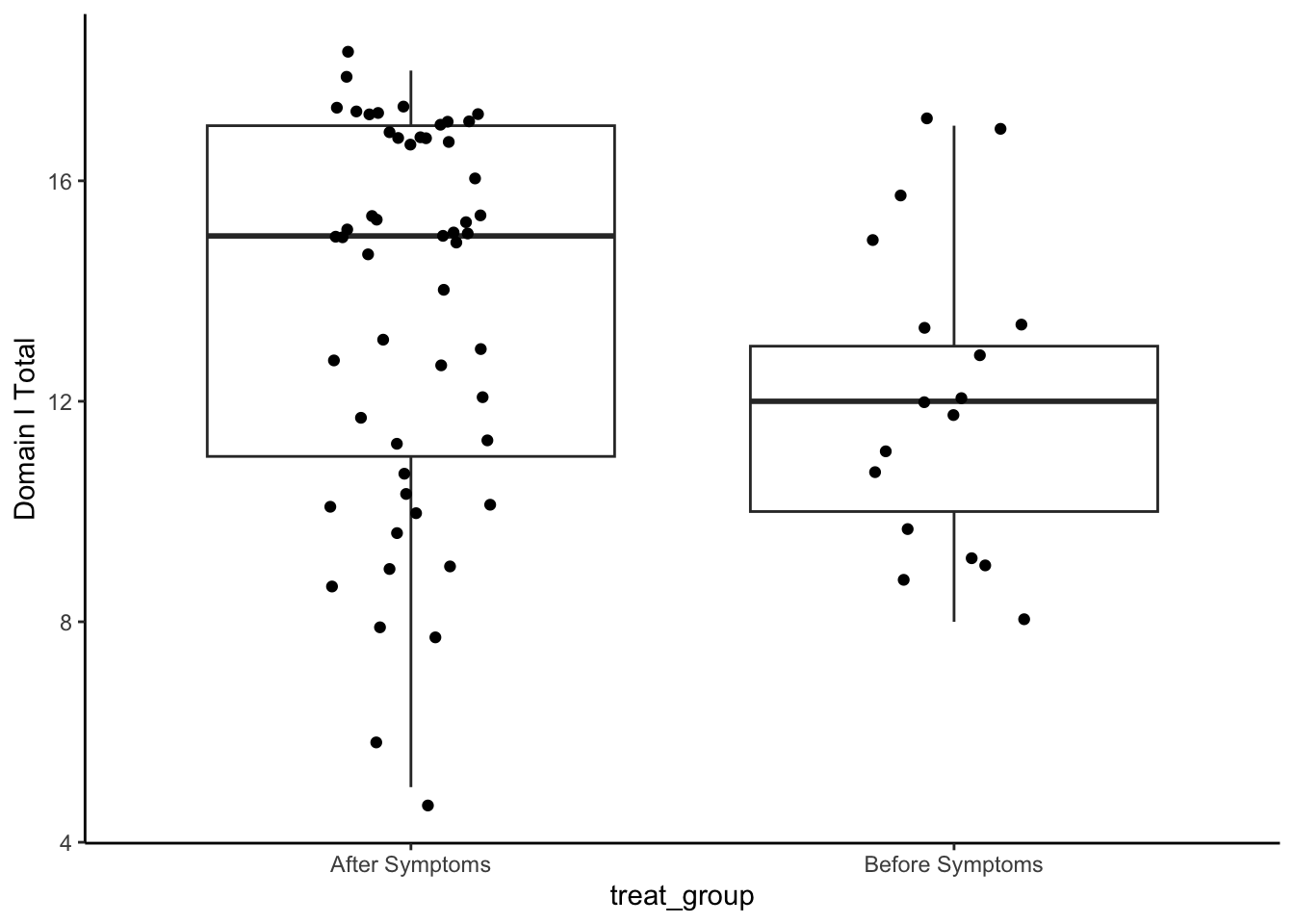
Medians and IQR
analysis_included_lastexam %>%
  group_by(treat_group) %>%
  summarize(Median = median(oi_domainI, na.rm=T),
            IQR = IQR(oi_domainI, na.rm=T),
            N = n()) %>%
kable(digits = 2)| treat_group | Median | IQR | N |
|---|---|---|---|
| After Symptoms | 15 | 6 | 52 |
| Before Symptoms | 12 | 3 | 17 |
Domain II: Palatal-Pharyngeal Approximation
set.seed(1234)
np.loc.test(x = analysis_included_last_b$oi_domainII,
            y = analysis_included_last_a$oi_domainII,
            alternative = "two.sided",
            median.test = TRUE,
            paired = FALSE,
            var.equal = FALSE)
Nonparametric Location Test (Studentized Wilcoxon Test)
alternative hypothesis: true median of differences is not equal to 0
t = -3.6569,  p-value = 0.0026
sample estimate:
median of the differences
                       -1
cliff.delta(analysis_included_last_b$oi_domainII, analysis_included_last_a$oi_domainII)
Cliff's Delta

delta estimate: -0.4128959 (medium)
95 percent confidence interval:
     lower      upper
-0.6063728 -0.1732641
Plot
analysis_included_lastexam %>%
  ggplot(aes(x = treat_group, y = oi_domainII)) +
  geom_boxplot() +
  geom_point(position = position_jitter(width = .15)) +
  labs(y = "Domain II Total")+
  theme_classic()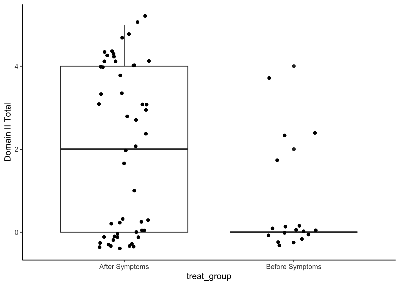
Medians and IQR
analysis_included_lastexam %>%
  group_by(treat_group) %>%
  summarize(Median = median(oi_domainII, na.rm=T),
            IQR = IQR(oi_domainII, na.rm=T),
            N = n()) %>%
kable(digits = 2)| treat_group | Median | IQR | N |
|---|---|---|---|
| After Symptoms | 2 | 4 | 52 |
| Before Symptoms | 0 | 0 | 17 |
Domain III: Airway Invasion/Laryngeal Closure
set.seed(1234)
np.loc.test(x = analysis_included_last_b$oi_domainIII,
            y = analysis_included_last_a$oi_domainIII,
            alternative = "two.sided",
            median.test = TRUE,
            paired = FALSE,
            var.equal = FALSE)
Nonparametric Location Test (Studentized Wilcoxon Test)
alternative hypothesis: true median of differences is not equal to 0
t = -4.4453,  p-value = 7e-04
sample estimate:
median of the differences
                       -2
cliff.delta(analysis_included_last_b$oi_domainIII, analysis_included_last_a$oi_domainIII)
Cliff's Delta

delta estimate: -0.5247982 (large)
95 percent confidence interval:
     lower      upper
-0.7164826 -0.2594309
Plot
analysis_included_lastexam %>%
  ggplot(aes(x = treat_group, y = oi_domainIII)) +
  geom_boxplot() +
  geom_point(position = position_jitter(width = .15)) +
  labs(y = "Domain III Total")+
  theme_classic()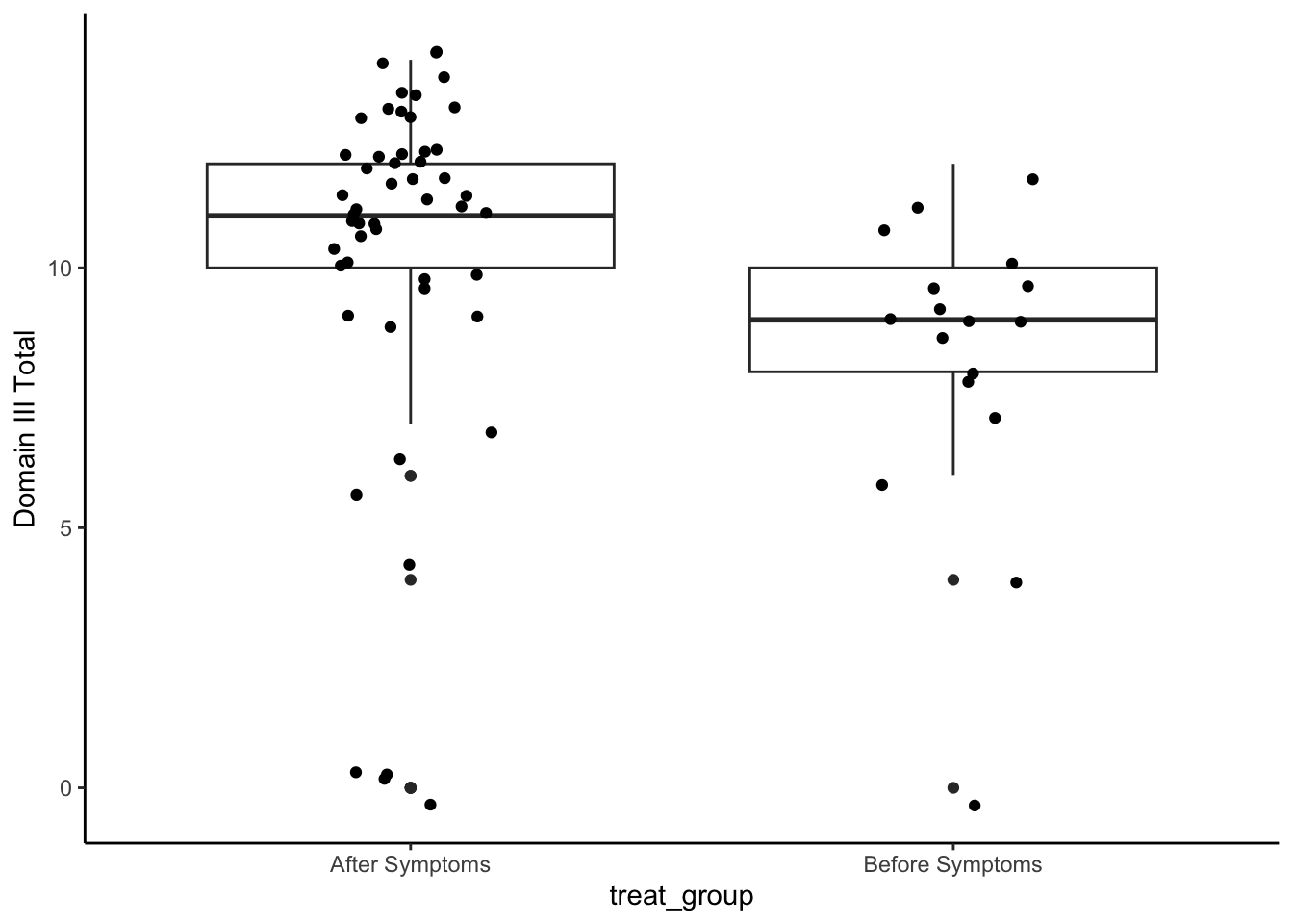
Medians and IQR
analysis_included_lastexam %>%
  group_by(treat_group) %>%
  summarize(Median = median(oi_domainIII, na.rm=T),
            IQR = IQR(oi_domainIII, na.rm=T),
            N = n()) %>%
kable(digits = 2)| treat_group | Median | IQR | N |
|---|---|---|---|
| After Symptoms | 11 | 2 | 52 |
| Before Symptoms | 9 | 2 | 17 |
Domain IV: Aspiration
set.seed(1234)
np.loc.test(x = analysis_included_last_b$oi_domainIV,
            y = analysis_included_last_a$oi_domainIV,
            alternative = "two.sided",
            median.test = TRUE,
            paired = FALSE,
            var.equal = FALSE)
Nonparametric Location Test (Studentized Wilcoxon Test)
alternative hypothesis: true median of differences is not equal to 0
t = -3.2465,  p-value = 0.0051
sample estimate:
median of the differences
                       -1
cliff.delta(analysis_included_last_b$oi_domainIV, analysis_included_last_a$oi_domainIV)
Cliff's Delta

delta estimate: -0.4232987 (medium)
95 percent confidence interval:
     lower      upper
-0.6423033 -0.1403899
Plot
analysis_included_lastexam %>%
  ggplot(aes(x = treat_group, y = oi_domainIV)) +
  geom_boxplot() +
  geom_point(position = position_jitter(width = .15)) +
  labs(y = "Domain IV Total")+
  theme_classic()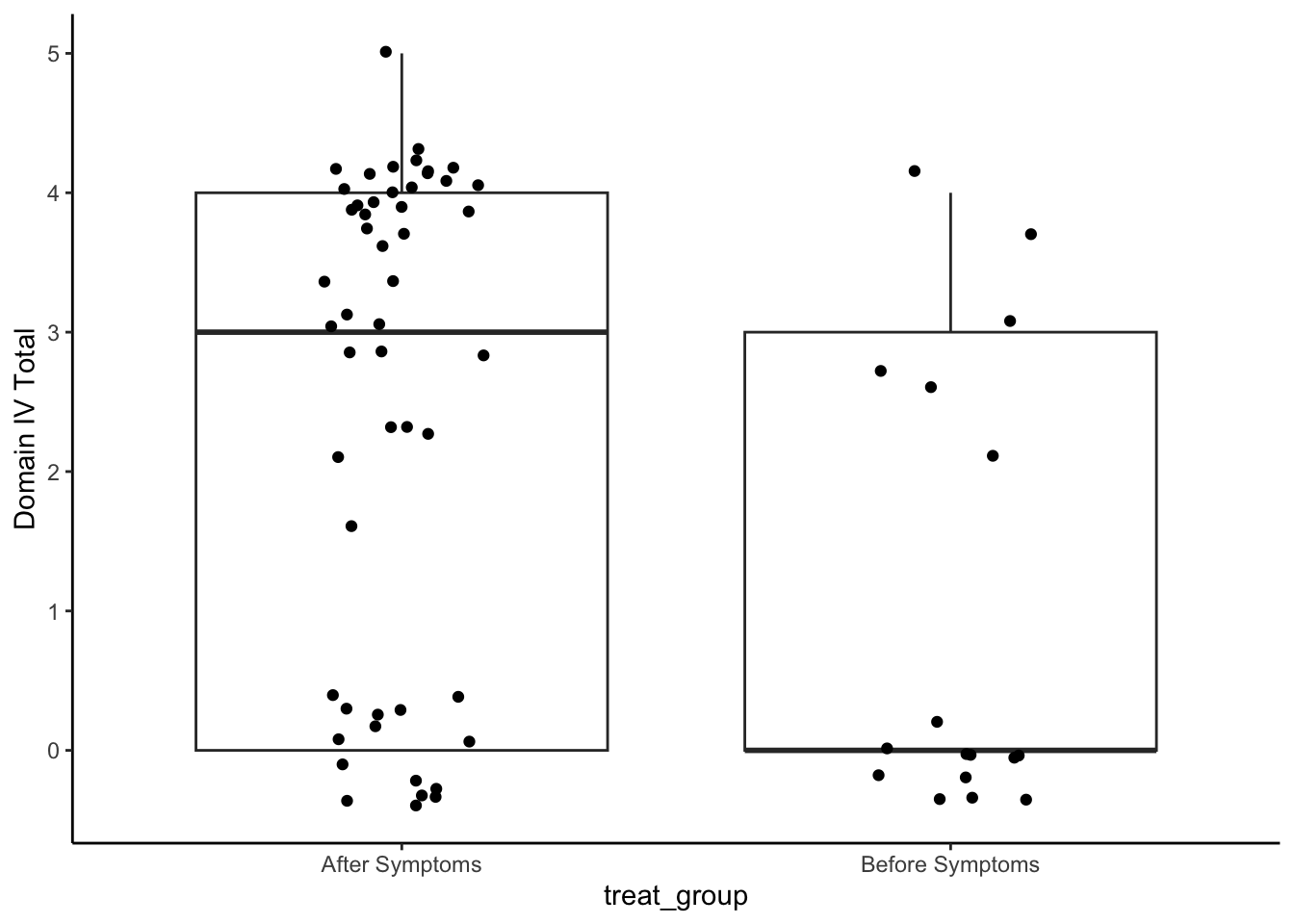
Medians and IQR
analysis_included_lastexam %>%
  group_by(treat_group) %>%
  summarize(Median = median(oi_domainIV, na.rm=T),
            IQR = IQR(oi_domainIV, na.rm=T),
            N = n()) %>%
kable(digits = 2)| treat_group | Median | IQR | N |
|---|---|---|---|
| After Symptoms | 3 | 4 | 52 |
| Before Symptoms | 0 | 3 | 17 |
Domain V: Pharyngeal Transport and Clearance
set.seed(1234)
np.loc.test(x = analysis_included_last_b$oi_domainV,
            y = analysis_included_last_a$oi_domainV,
            alternative = "two.sided",
            median.test = TRUE,
            paired = FALSE,
            var.equal = FALSE)
Nonparametric Location Test (Studentized Wilcoxon Test)
alternative hypothesis: true median of differences is not equal to 0
t = -6.0216,  p-value = 2e-04
sample estimate:
median of the differences
                       -4
cliff.delta(analysis_included_last_b$oi_domainV, analysis_included_last_a$oi_domainV)
Cliff's Delta

delta estimate: -0.6346154 (large)
95 percent confidence interval:
     lower      upper
-0.8062500 -0.3644367
Plot
analysis_included_lastexam %>%
  ggplot(aes(x = treat_group, y = oi_domainV)) +
  geom_boxplot() +
  geom_point(position = position_jitter(width = .15)) +
  labs(y = "Domain V Total")+
  theme_classic()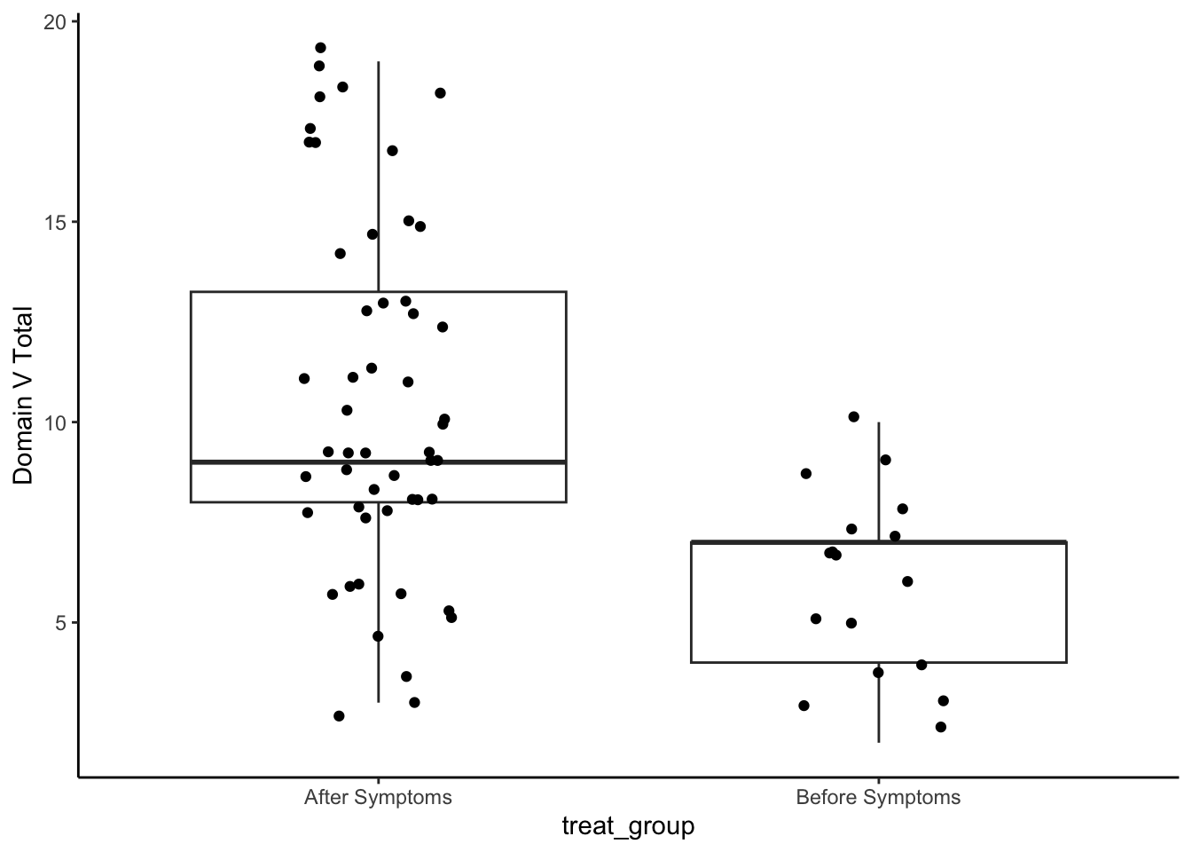
Medians and IQR
analysis_included_lastexam %>%
  group_by(treat_group) %>%
  summarize(Median = median(oi_domainV, na.rm=T),
            IQR = IQR(oi_domainV, na.rm=T),
            N = n()) %>%
kable(digits = 2)| treat_group | Median | IQR | N |
|---|---|---|---|
| After Symptoms | 9 | 5.25 | 52 |
| Before Symptoms | 7 | 3.00 | 17 |
Question: What are the functional differences in impariment in last exam between patients treated before vs after sypmtoms?
analysis_included_lastexam <- analysis_included_lastexam %>%
  mutate(resp_cur___1c = ifelse(resp_cur___1 == 1, "None", ""),
         resp_cur___2c = ifelse(resp_cur___2 == 1, "BiPAP, Wake & Nocturnal", ""),
         resp_cur___3c = ifelse(resp_cur___3 == 1, "BiPAP, Nocturnal", ""),
         resp_cur___4c = ifelse(resp_cur___4 == 1, "Oxygen via Nasal Canula",""),
         resp_cur___5c = ifelse(resp_cur___5 == 1, "Tracheostomy",""),
         resp_cur___6c = ifelse(resp_cur___6 == 1, "Ventilator, Continuous", ""),
         resp_cur___7c = ifelse(resp_cur___7 == 1, "Ventilator, Nocturnal", ""),
         secretions_comb = ifelse(secretions___2 == 1, "Suctioning needed", "Managing secretions"))


analysis_included_lastexam$resp_cur_comb <- apply(analysis_included_lastexam[,c("resp_cur___1c", "resp_cur___2c", "resp_cur___3c", "resp_cur___4c", "resp_cur___5c", "resp_cur___6c", "resp_cur___7c")], 1, function(x) paste(x[x != ""], collapse=" & "))

analysis_included_lastexam$resp_text_any <- ifelse(grepl("BiPAP|Ventilator", analysis_included_lastexam$resp_cur_comb), "BiPAP or Ventilator", "None")
Is the patient currently managing their own secretions?
analysis_included_lastexam %>%
  group_by(treat_group, secretions_comb) %>%
  summarize(count=n()) %>%
  group_by(treat_group) %>%
  mutate(Percent = count/sum(count)*100) %>%
  arrange(treat_group, desc(count)) %>%
  kable(col.names = c("Treatment Group", "Secretions Last Exam", "Count", "Percent"),
digits=2)| Treatment Group | Secretions Last Exam | Count | Percent |
|---|---|---|---|
| After Symptoms | Managing secretions | 32 | 61.54 |
| After Symptoms | Suctioning needed | 20 | 38.46 |
| Before Symptoms | Managing secretions | 17 | 100.00 |
Does secretion management for last exam differ between groups?
table_sec_last <- table(analysis_included_lastexam$secretions_comb, analysis_included_lastexam$treat_group)

analysis_included_lastexam %>%
  group_by(treat_group, secretions_comb) %>%
  tally() %>%
  pivot_wider(names_from = treat_group,
              values_from = n,
              values_fill = 0) %>%
kable()| secretions_comb | After Symptoms | Before Symptoms |
|---|---|---|
| Managing secretions | 32 | 17 |
| Suctioning needed | 20 | 0 |
#chisq.test(table_sec_last)

fisher.test(table_sec_last)
    Fisher's Exact Test for Count Data

data:  table_sec_last
p-value = 0.001527
alternative hypothesis: true odds ratio is not equal to 1
95 percent confidence interval:
 0.000000 0.450985
sample estimates:
odds ratio
         0
# #odds ratio (Odds Yes in After /Odds Yes in Before)
# (table_sec_last["Suctioning needed", "After Symptoms"]/table_sec_last["Managing secretions", "After Symptoms"])/(table_sec_last["Suctioning needed", "Before Symptoms"]/table_sec_last["Managing secretions", "Before Symptoms"])What are the patient’s respiratory supports for the last exam?
analysis_included_lastexam %>%
  group_by(treat_group, resp_cur_comb) %>%
  summarize(count=n()) %>%
  group_by(treat_group) %>%
  mutate(Percent = count/sum(count)*100) %>%
  arrange(treat_group, desc(count)) %>%
  kable(col.names = c("Treatment Group", "Respiratory support", "Count", "Percent"),
digits=2)| Treatment Group | Respiratory support | Count | Percent |
|---|---|---|---|
| After Symptoms | None | 23 | 44.23 |
| After Symptoms | BiPAP, Nocturnal | 22 | 42.31 |
| After Symptoms | BiPAP, Wake & Nocturnal | 2 | 3.85 |
| After Symptoms | Oxygen via Nasal Canula | 2 | 3.85 |
| After Symptoms | Tracheostomy & Ventilator, Continuous | 2 | 3.85 |
| After Symptoms | BiPAP, Nocturnal & Oxygen via Nasal Canula | 1 | 1.92 |
| Before Symptoms | None | 16 | 94.12 |
| Before Symptoms | BiPAP, Nocturnal | 1 | 5.88 |
Do kinds of support differ between groups?
For this, will use chi-squared tests, with collapsed groups to meet expected values assumptions
table_resp_group_last1 <- table(analysis_included_lastexam$resp_text_any, analysis_included_lastexam$treat_group)

analysis_included_lastexam %>%
  group_by(treat_group, resp_text_any) %>%
  tally() %>%
  pivot_wider(names_from = treat_group,
              values_from = n,
              values_fill = 0) %>%
kable()| resp_text_any | After Symptoms | Before Symptoms |
|---|---|---|
| BiPAP or Ventilator | 27 | 1 |
| None | 25 | 16 |
chisq.test(table_resp_group_last1)
    Pearson's Chi-squared test with Yates' continuity correction

data:  table_resp_group_last1
X-squared = 9.4343, df = 1, p-value = 0.00213
#calculate odds ratio (Odds Yes in After /Odds Yes in Before)
(table_resp_group_last1["BiPAP or Ventilator", "After Symptoms"]/table_resp_group_last1["None", "After Symptoms"])/(table_resp_group_last1["BiPAP or Ventilator", "Before Symptoms"]/table_resp_group_last1["None", "Before Symptoms"])[1] 17.28What is the patient’s current oral intake regimen (FOIS)?
Note: Only taking the current FOIS data (“fois_cur”) for last exam, with the exception of NZ_11 who only has values in “fois_past”.
#use past fois value for current in NZ_11 (otherwise NA)
analysis_included_lastexam$fois_cur[which(analysis_included_lastexam$Subject.ID == "NZ_11")] <- analysis_included_lastexam$fois_past[which(analysis_included_lastexam$Subject.ID == "NZ_11")]
analysis_included_lastexam <- analysis_included_lastexam %>%
mutate(fois_curc = case_when(fois_cur == 1 ~ "1-No liquids/foods by mouth",
fois_cur == 2 ~ "2-Tube dependent, minimal attempts at liquids/foods",
fois_cur == 3 ~ "3-Tube dependent, consistent intake of liquids/foods",
fois_cur == 4 ~ "4-Total oral diet, requiring special preparation of liquids (ie thickening)",
fois_cur == 7 ~ "7-Total oral diet, requiring special preparations of solids (ie dierent textures/liquid supplements)",
fois_cur == 5 ~ "5-Total oral diet without special preparations but with compensations (ie strategies/feeding equipment)",
fois_cur == 6 ~ "6-Total oral diet, no restrictions"),
fois_cur_collapsed = case_when(fois_cur == 1 ~ "Tube dependent",
fois_cur == 2 ~ "Tube dependent",
fois_cur == 3 ~ "Tube dependent",
fois_cur == 4 ~ "Total oral diet",
fois_cur == 7 ~ "Total oral diet",
fois_cur == 5 ~ "Total oral diet",
fois_cur == 6 ~ "Total oral diet"),
fois_15_6 = ifelse(fois_cur <= 5 | fois_cur == 7, "FOIS 1-5", "FOIS 6"),
fois_imp = ifelse(fois_cur < 4, "Yes", "No"))
analysis_included_lastexam %>%
group_by(treat_group, fois_curc) %>%
summarize(count=n()) %>%
group_by(treat_group) %>%
mutate(Percent = count/sum(count)*100) %>%
arrange(treat_group) %>%
kable(col.names = c("Treatment Group", "FOIS", "Count", "Percent"),
digits=2)| Treatment Group | FOIS | Count | Percent |
|---|---|---|---|
| After Symptoms | 1-No liquids/foods by mouth | 10 | 19.23 |
| After Symptoms | 2-Tube dependent, minimal attempts at liquids/foods | 7 | 13.46 |
| After Symptoms | 3-Tube dependent, consistent intake of liquids/foods | 9 | 17.31 |
| After Symptoms | 4-Total oral diet, requiring special preparation of liquids (ie thickening) | 5 | 9.62 |
| After Symptoms | 5-Total oral diet without special preparations but with compensations (ie strategies/feeding equipment) | 7 | 13.46 |
| After Symptoms | 6-Total oral diet, no restrictions | 14 | 26.92 |
| Before Symptoms | 3-Tube dependent, consistent intake of liquids/foods | 2 | 11.76 |
| Before Symptoms | 6-Total oral diet, no restrictions | 15 | 88.24 |
Does FOIS differ between groups?
Compare proportion of kids in FOIS 1-5 (including coded as 7, which should be = 4.5) for each group
Grouped (e.g., 1-5 vs 6)
table_fois_last_156 <- table(analysis_included_lastexam$fois_15_6, analysis_included_lastexam$treat_group)


analysis_included_lastexam %>%
  group_by(treat_group, fois_15_6) %>%
  tally() %>%
  pivot_wider(names_from = treat_group,
              values_from = n,
              values_fill = 0) %>%
kable()| fois_15_6 | After Symptoms | Before Symptoms |
|---|---|---|
| FOIS 1-5 | 38 | 2 |
| FOIS 6 | 14 | 15 |
chisq.test(table_fois_last_156)
    Pearson's Chi-squared test with Yates' continuity correction

data:  table_fois_last_156
X-squared = 17.33, df = 1, p-value = 3.141e-05
#odds ratio (Odds Yes in After /Odds Yes in Before)
(table_fois_last_156["FOIS 1-5", "After Symptoms"]/table_fois_last_156["FOIS 6", "After Symptoms"])/(table_fois_last_156["FOIS 1-5", "Before Symptoms"]/table_fois_last_156["FOIS 6", "Before Symptoms"])[1] 20.35714Individually?
analysis_included_lastexam %>%
  group_by(treat_group, fois_curc) %>%
  tally() %>%
  pivot_wider(names_from = treat_group,
              values_from = n,
              values_fill = 0) %>%
kable()| fois_curc | After Symptoms | Before Symptoms |
|---|---|---|
| 1-No liquids/foods by mouth | 10 | 0 |
| 2-Tube dependent, minimal attempts at liquids/foods | 7 | 0 |
| 3-Tube dependent, consistent intake of liquids/foods | 9 | 2 |
| 4-Total oral diet, requiring special preparation of liquids (ie thickening) | 5 | 0 |
| 5-Total oral diet without special preparations but with compensations (ie strategies/feeding equipment) | 7 | 0 |
| 6-Total oral diet, no restrictions | 14 | 15 |
Proportion of Kids with Profound Impairments at last exam By Treatment before vs After Symptoms
For each of the components, will identify the proportion of kids who exhibited profound impairments.
Create impairment scores
analysis_included_lastexam <- analysis_included_lastexam %>%
  mutate(oi_21_imp = ifelse(oi_21 == 2 | oi_21 == 3, "Yes", "No"),
         oi_20_imp = ifelse(oi_20 == 3 | oi_20 == 4, "Yes", "No"),
         oi_18_imp = ifelse(oi_18 == 2, "Yes", "No"),
         oi_17_imp = ifelse(oi_17 == 3 | oi_17 == 4, "Yes", "No"),
         oi_14_imp = ifelse(oi_14 == 1 | oi_14 == 2, "Yes", "No"),
         oi_12_imp = ifelse(oi_12 == 1 | oi_12 == 2, "Yes", "No"),
         oi_8_imp = ifelse(oi_8 == 2, "Yes", "No"),
         oi_10_imp = ifelse(oi_10 == 2 | oi_10 == 3, "Yes", "No"),
         oi_7_imp = ifelse(oi_7 == 2 | oi_7 == 3, "Yes", "No"),
         oi_2_imp = ifelse(oi_2 == 7, "Yes", "No"),
         oi_19_imp = ifelse(oi_19 > 2, "Yes", "No"),
         oi_1_imp = ifelse(oi_1 == 2, "Yes", "No"),
         oi_1_0 = ifelse(oi_1 == 0, "Yes", "No"),
         sec_imp = ifelse(secretions___2 == 1, "Yes, suctioning needed", "No"),
         fois_imp = ifelse(fois_cur < 4, "Yes", "No"))
OI_1
Proportion with a 2 or not by treatment group
analysis_included_lastexam %>%
  filter(!is.na(oi_1)) %>%
  group_by(treat_group, oi_1_imp) %>%
  tally() %>%
  group_by(treat_group) %>%
  mutate(percent = n/sum(n)*100) %>%
  pivot_wider(names_from = treat_group,
              values_from = c(n, percent),
              names_vary = "slowest",
              values_fill = 0) %>%
kable(digits=2)| oi_1_imp | n_After Symptoms | percent_After Symptoms | n_Before Symptoms | percent_Before Symptoms |
|---|---|---|---|---|
| No | 24 | 46.15 | 13 | 76.47 |
| Yes | 28 | 53.85 | 4 | 23.53 |
Chi-squared to test whether different
oi1_imptb_last <- table(analysis_included_lastexam$treat_group, analysis_included_lastexam$oi_1_imp)

chisq.test(oi1_imptb_last)
    Pearson's Chi-squared test with Yates' continuity correction

data:  oi1_imptb_last
X-squared = 3.5943, df = 1, p-value = 0.05798
Look at scores of 0 in each group
analysis_included_lastexam %>%
  filter(!is.na(oi_1)) %>%
  group_by(treat_group, oi_1_0) %>%
  tally() %>%
  group_by(treat_group) %>%
  mutate(percent = n/sum(n)*100) %>%
  pivot_wider(names_from = treat_group,
              values_from = c(n, percent),
              names_vary = "slowest",
              values_fill = 0) %>%
kable(digits=2)| oi_1_0 | n_After Symptoms | percent_After Symptoms | n_Before Symptoms | percent_Before Symptoms |
|---|---|---|---|---|
| No | 31 | 59.62 | 5 | 29.41 |
| Yes | 21 | 40.38 | 12 | 70.59 |
Chi-squared to test whether different
oi1_0_last <- table(analysis_included_lastexam$oi_1_0, analysis_included_lastexam$treat_group)

chisq.test(oi1_0_last)
    Pearson's Chi-squared test with Yates' continuity correction

data:  oi1_0_last
X-squared = 3.5516, df = 1, p-value = 0.05949
#odds ratio (Odds Yes in After /Odds Yes in Before)
(oi1_0_last["Yes", "After Symptoms"]/oi1_0_last["No", "After Symptoms"])/(oi1_0_last["Yes", "Before Symptoms"]/oi1_0_last["No", "Before Symptoms"])[1] 0.2822581OI_2
Proportion with a 7 or not by treatment group
analysis_included_lastexam %>%
  filter(!is.na(oi_2)) %>%
  group_by(treat_group, oi_2_imp) %>%
  tally() %>%
  group_by(treat_group) %>%
  mutate(percent = n/sum(n)*100) %>%
  pivot_wider(names_from = treat_group,
              values_from = c(n, percent),
              names_vary = "slowest",
              values_fill = 0) %>%
kable(digits=2)| oi_2_imp | n_After Symptoms | percent_After Symptoms | n_Before Symptoms | percent_Before Symptoms |
|---|---|---|---|---|
| No | 23 | 44.23 | 13 | 76.47 |
| Yes | 29 | 55.77 | 4 | 23.53 |
Chi-squared to test whether different
oi2_imptb_last <- table(analysis_included_lastexam$treat_group, analysis_included_lastexam$oi_2_imp)

chisq.test(oi2_imptb_last)
    Pearson's Chi-squared test with Yates' continuity correction

data:  oi2_imptb_last
X-squared = 4.1228, df = 1, p-value = 0.04231
OI_7
Proportion with a 2 or 3 or not by group
analysis_included_lastexam %>%
  filter(!is.na(oi_7)) %>%
  group_by(treat_group, oi_7_imp) %>%
  tally() %>%
  group_by(treat_group) %>%
  mutate(percent = n/sum(n)*100) %>%
  pivot_wider(names_from = treat_group,
              values_from = c(n, percent),
              names_vary = "slowest",
              values_fill = 0) %>%
kable(digits=2)| oi_7_imp | n_After Symptoms | percent_After Symptoms | n_Before Symptoms | percent_Before Symptoms |
|---|---|---|---|---|
| No | 30 | 57.69 | 16 | 94.12 |
| Yes | 22 | 42.31 | 1 | 5.88 |
Chi-squared to test whether different
oi7_imptb_last <- table(analysis_included_lastexam$treat_group, analysis_included_lastexam$oi_7_imp)

chisq.test(oi7_imptb_last)
    Pearson's Chi-squared test with Yates' continuity correction

data:  oi7_imptb_last
X-squared = 6.098, df = 1, p-value = 0.01353
OI_8
Proportion with a 2 or not by group
analysis_included_lastexam %>%
  filter(!is.na(oi_8)) %>%
  group_by(treat_group, oi_8_imp) %>%
  tally() %>%
  group_by(treat_group) %>%
  mutate(percent = n/sum(n)*100) %>%
  pivot_wider(names_from = treat_group,
              values_from = c(n, percent),
              names_vary = "slowest",
              values_fill = 0) %>%
kable(digits=2)| oi_8_imp | n_After Symptoms | percent_After Symptoms | n_Before Symptoms | percent_Before Symptoms |
|---|---|---|---|---|
| No | 32 | 61.54 | 16 | 94.12 |
| Yes | 20 | 38.46 | 1 | 5.88 |
Chi-squared to test whether different
oi8_imptb_last <- table(analysis_included_lastexam$treat_group, analysis_included_lastexam$oi_8_imp)

chisq.test(oi8_imptb_last)
    Pearson's Chi-squared test with Yates' continuity correction

data:  oi8_imptb_last
X-squared = 4.9761, df = 1, p-value = 0.0257
OI_10
Proportion with a 2 or 3 or not by group
analysis_included_lastexam %>%
  filter(!is.na(oi_10_imp)) %>%
  group_by(treat_group, oi_10_imp) %>%
  tally() %>%
  group_by(treat_group) %>%
  mutate(percent = n/sum(n)*100) %>%
  pivot_wider(names_from = treat_group,
              values_from = c(n, percent),
              names_vary = "slowest",
              values_fill = 0) %>%
kable(digits=2)| oi_10_imp | n_After Symptoms | percent_After Symptoms | n_Before Symptoms | percent_Before Symptoms |
|---|---|---|---|---|
| No | 28 | 54.9 | 17 | 100 |
| Yes | 23 | 45.1 | 0 | 0 |
Chi-squared to test whether different
oi10_imptb_last <- table(analysis_included_lastexam$treat_group, analysis_included_lastexam$oi_10_imp)

chisq.test(oi10_imptb_last)
    Pearson's Chi-squared test with Yates' continuity correction

data:  oi10_imptb_last
X-squared = 9.658, df = 1, p-value = 0.001885
OI_12
Proportion with a 1 or 2 or not by group
analysis_included_lastexam %>%
  filter(!is.na(oi_12)) %>%
  group_by(treat_group, oi_12_imp) %>%
  tally() %>%
  group_by(treat_group) %>%
  mutate(percent = n/sum(n)*100) %>%
  pivot_wider(names_from = treat_group,
              values_from = c(n, percent),
              names_vary = "slowest",
              values_fill = 0) %>%
kable(digits=2)| oi_12_imp | n_After Symptoms | percent_After Symptoms | n_Before Symptoms | percent_Before Symptoms |
|---|---|---|---|---|
| No | 4 | 7.84 | 1 | 5.88 |
| Yes | 47 | 92.16 | 16 | 94.12 |
Chi-squared to test whether different (using Fisher here because of small expected counts)
oi12_imptb_last <- table(analysis_included_lastexam$treat_group, analysis_included_lastexam$oi_12_imp)

fisher.test(oi12_imptb_last)
    Fisher's Exact Test for Count Data

data:  oi12_imptb_last
p-value = 1
alternative hypothesis: true odds ratio is not equal to 1
95 percent confidence interval:
  0.1218223 71.1718451
sample estimates:
odds ratio
  1.355913
OI_14
Proportion with a 1 or 2 or not by group
analysis_included_lastexam %>%
  filter(!is.na(oi_14)) %>%
  group_by(treat_group, oi_14_imp) %>%
  tally() %>%
  group_by(treat_group) %>%
  mutate(percent = n/sum(n)*100) %>%
  pivot_wider(names_from = treat_group,
              values_from = c(n, percent),
              names_vary = "slowest",
              values_fill = 0) %>%
kable(digits=2)| oi_14_imp | n_After Symptoms | percent_After Symptoms | n_Before Symptoms | percent_Before Symptoms |
|---|---|---|---|---|
| No | 15 | 29.41 | 11 | 64.71 |
| Yes | 36 | 70.59 | 6 | 35.29 |
Chi-squared to test whether different
oi14_imptb_last <- table(analysis_included_lastexam$oi_14_imp, analysis_included_lastexam$treat_group)

chisq.test(oi14_imptb_last)
    Pearson's Chi-squared test with Yates' continuity correction

data:  oi14_imptb_last
X-squared = 5.3138, df = 1, p-value = 0.02116
#odds ratio (Odds Yes in After /Odds Yes in Before)
(oi14_imptb_last["Yes", "After Symptoms"]/oi14_imptb_last["No", "After Symptoms"])/(oi14_imptb_last["Yes", "Before Symptoms"]/oi14_imptb_last["No", "Before Symptoms"])[1] 4.4Look at referral reason for those who aspirated
analysis_included_lastexam %>%
  filter(oi_14_imp == "Yes") %>%
  group_by(referralc, treat_group) %>%
  tally() %>%
  group_by(treat_group) %>%
  mutate(percent = n/sum(n)*100) %>%
  pivot_wider(names_from = treat_group,
              values_from = c(n, percent),
              names_vary = "slowest",
              values_fill = 0) %>%
kable(digits=2)| referralc | n_After Symptoms | percent_After Symptoms | n_Before Symptoms | percent_Before Symptoms |
|---|---|---|---|---|
| Asymptomatic, Standard High Risk Referral at Diagnosis | 3 | 8.33 | 4 | 66.67 |
| Caregiver reported symptoms | 7 | 19.44 | 1 | 16.67 |
| Concerns that swallowing may be contributing to nutritional or respiratory impairments given high risk | 11 | 30.56 | 1 | 16.67 |
| Follow-Up from previous impairment | 15 | 41.67 | 0 | 0.00 |
OI_17
Proportion with a 3 or 4 or not by group
analysis_included_lastexam %>%
  filter(!is.na(oi_17)) %>%
  group_by(treat_group, oi_17_imp) %>%
  tally() %>%
  group_by(treat_group) %>%
  mutate(percent = n/sum(n)*100) %>%
  pivot_wider(names_from = treat_group,
              values_from = c(n, percent),
              names_vary = "slowest",
              values_fill = 0) %>%
kable(digits=2)| oi_17_imp | n_After Symptoms | percent_After Symptoms | n_Before Symptoms | percent_Before Symptoms |
|---|---|---|---|---|
| No | 32 | 61.54 | 17 | 100 |
| Yes | 20 | 38.46 | 0 | 0 |
Chi-squared to test whether different
oi17_imptb_last <- table(analysis_included_lastexam$treat_group, analysis_included_lastexam$oi_17_imp)

chisq.test(oi17_imptb_last)
    Pearson's Chi-squared test with Yates' continuity correction

data:  oi17_imptb_last
X-squared = 7.4335, df = 1, p-value = 0.006402
OI_18
Proportion with a 2 or not by group
analysis_included_lastexam %>%
  filter(!is.na(oi_18)) %>%
  group_by(treat_group, oi_18_imp) %>%
  tally() %>%
  group_by(treat_group) %>%
  mutate(percent = n/sum(n)*100) %>%
  pivot_wider(names_from = treat_group,
              values_from = c(n, percent),
              names_vary = "slowest",
              values_fill = 0) %>%
kable(digits=2)| oi_18_imp | n_After Symptoms | percent_After Symptoms | n_Before Symptoms | percent_Before Symptoms |
|---|---|---|---|---|
| No | 42 | 80.77 | 16 | 94.12 |
| Yes | 10 | 19.23 | 1 | 5.88 |
Chi-squared to test whether different
oi18_imptb_last <- table(analysis_included_lastexam$treat_group, analysis_included_lastexam$oi_18_imp)

#chisq.test(oi18_imptb_last)

#use fishers for small expected counts
fisher.test(oi18_imptb_last)
    Fisher's Exact Test for Count Data

data:  oi18_imptb_last
p-value = 0.2705
alternative hypothesis: true odds ratio is not equal to 1
95 percent confidence interval:
 0.005702566 2.158791039
sample estimates:
odds ratio
 0.2663952
OI_19
Proportion above a 2 or not by group
analysis_included_lastexam %>%
  filter(!is.na(oi_19)) %>%
  group_by(treat_group, oi_19_imp) %>%
  tally() %>%
  group_by(treat_group) %>%
  mutate(percent = n/sum(n)*100) %>%
  pivot_wider(names_from = treat_group,
              values_from = c(n, percent),
              names_vary = "slowest",
              values_fill = 0) %>%
kable(digits=2)| oi_19_imp | n_After Symptoms | percent_After Symptoms | n_Before Symptoms | percent_Before Symptoms |
|---|---|---|---|---|
| No | 34 | 65.38 | 17 | 100 |
| Yes | 18 | 34.62 | 0 | 0 |
Chi-squared to test whether different
oi19_imptb_last <- table(analysis_included_lastexam$treat_group, analysis_included_lastexam$oi_19_imp)

chisq.test(oi19_imptb_last)
    Pearson's Chi-squared test with Yates' continuity correction

data:  oi19_imptb_last
X-squared = 6.2675, df = 1, p-value = 0.0123
OI_20
Proportion with a 3 or 4 or not by group
analysis_included_lastexam %>%
  filter(!is.na(oi_20)) %>%
  group_by(treat_group, oi_20_imp) %>%
  tally() %>%
  group_by(treat_group) %>%
  mutate(percent = n/sum(n)*100) %>%
  pivot_wider(names_from = treat_group,
              values_from = c(n, percent),
              names_vary = "slowest",
              values_fill = 0) %>%
kable(digits=2)| oi_20_imp | n_After Symptoms | percent_After Symptoms | n_Before Symptoms | percent_Before Symptoms |
|---|---|---|---|---|
| No | 35 | 67.31 | 17 | 100 |
| Yes | 17 | 32.69 | 0 | 0 |
Chi-squared to test whether different
oi20_imptb_last <- table(analysis_included_lastexam$treat_group, analysis_included_lastexam$oi_20_imp)

chisq.test(oi20_imptb_last)
    Pearson's Chi-squared test with Yates' continuity correction

data:  oi20_imptb_last
X-squared = 5.719, df = 1, p-value = 0.01678
OI_21
Proportion with a 2 or 3 or not by group
analysis_included_lastexam %>%
  filter(!is.na(oi_21)) %>%
  group_by(treat_group, oi_21_imp) %>%
  tally() %>%
  group_by(treat_group) %>%
  mutate(percent = n/sum(n)*100) %>%
  pivot_wider(names_from = treat_group,
              values_from = c(n, percent),
              names_vary = "slowest",
              values_fill = 0) %>%
kable(digits=2)| oi_21_imp | n_After Symptoms | percent_After Symptoms | n_Before Symptoms | percent_Before Symptoms |
|---|---|---|---|---|
| No | 33 | 63.46 | 16 | 94.12 |
| Yes | 19 | 36.54 | 1 | 5.88 |
Chi-squared to test whether different
oi21_imptb_last <- table(analysis_included_lastexam$oi_21_imp, analysis_included_lastexam$treat_group)

chisq.test(oi21_imptb_last)
    Pearson's Chi-squared test with Yates' continuity correction

data:  oi21_imptb_last
X-squared = 4.4548, df = 1, p-value = 0.0348
#odds ratio (Odds Yes in After /Odds Yes in Before)
(oi21_imptb_last["Yes", "After Symptoms"]/oi21_imptb_last["No", "After Symptoms"])/(oi21_imptb_last["Yes", "Before Symptoms"]/oi21_imptb_last["No", "Before Symptoms"])[1] 9.212121Which domains & components relate to functional outcomes?
Could test this using a point-biserial correlation (for domains + the binary variables of whether or not they show impairment) to see which domains are most associated with having impairments in the functional outcomes. Can also put all the domains into a logistic regression to look at prediction.
Recode to 0=no impariment; 1 = impairment
analysis_included_lastexam <- analysis_included_lastexam %>%
  mutate(sec_imp_n = ifelse(sec_imp == "No", 0, 1),
         fois_imp_n = ifelse(fois_imp == "No", 0, 1),
         resp_imp_n = ifelse(resp_text_any == "None", 0, 1),
         oi_17_imp_n = ifelse(oi_17_imp == "No", 0, 1),
         oi_18_imp_n = ifelse(oi_18_imp == "No", 0, 1))

# pcr_dat <- SMA_DAT %>%
#   filter(Measurement_name == "PCR")
#
Secreation management
Point-biserial associations (note: treats domain scores as continuous):
analysis_included_lastexam %>%
  select(sec_imp_n, contains("domain")) %>%
  pivot_longer(cols = contains("domain"),
               names_to = "domain",
               values_to = "score") %>%
  group_by(domain) %>%
  summarize(pb_correlation = cor(sec_imp_n, score, use="pairwise.complete.obs"),
            n = sum(!is.na(score)),
            p = cor.test(sec_imp_n, score)$p.value) %>%
kable(digits = 2)| domain | pb_correlation | n | p |
|---|---|---|---|
| oi_domainI | 0.37 | 69 | 0.00 |
| oi_domainII | 0.25 | 69 | 0.03 |
| oi_domainIII | 0.14 | 68 | 0.26 |
| oi_domainIV | 0.13 | 68 | 0.28 |
| oi_domainV | 0.49 | 69 | 0.00 |
Plots:
analysis_included_lastexam %>%
  select(sec_imp_n, contains("domain")) %>%
  pivot_longer(cols = contains("domain"),
               names_to = "domain",
               values_to = "score") %>%
  ggplot(aes(x = sec_imp_n, y = score)) +
    geom_point(position = position_jitter(width = .05)) +
    geom_smooth(method = "lm", se = F) +
    facet_wrap(~domain) +
    theme_classic()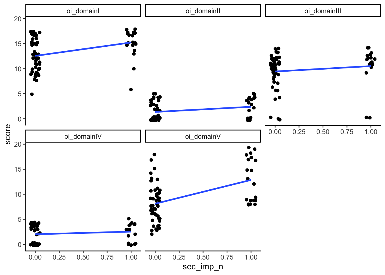
Logistic regressions
secdomain_logr <- glm(sec_imp_n ~ oi_domainI + oi_domainII + oi_domainIII + oi_domainIV + oi_domainV, family = "binomial", data = analysis_included_lastexam)

secdomain_logr %>%
  tidy() %>%
kable(digits = 3)| term | estimate | std.error | statistic | p.value |
|---|---|---|---|---|
| (Intercept) | -5.451 | 2.002 | -2.722 | 0.006 |
| oi_domainI | 0.185 | 0.128 | 1.440 | 0.150 |
| oi_domainII | -0.026 | 0.240 | -0.107 | 0.915 |
| oi_domainIII | -0.158 | 0.138 | -1.144 | 0.253 |
| oi_domainIV | 0.142 | 0.275 | 0.517 | 0.605 |
| oi_domainV | 0.304 | 0.110 | 2.757 | 0.006 |
Domain V is the only one significantly related to whether secretions would be impaired versus not. You can interpret the coefficient by taking the exponent of the estimate, 0.3035815, which is 1.354702.
FOIS
Point-biserial associations (note: treats domain scores as continuous):
analysis_included_lastexam %>%
  select(fois_imp_n, contains("domain")) %>%
  pivot_longer(cols = contains("domain"),
               names_to = "domain",
               values_to = "score") %>%
  group_by(domain) %>%
  summarize(pb_correlation = cor(fois_imp_n, score, use="pairwise.complete.obs"),
            n = sum(!is.na(score)),
            p = cor.test(fois_imp_n, score)$p.value) %>%
kable(digits = 2)| domain | pb_correlation | n | p |
|---|---|---|---|
| oi_domainI | 0.39 | 69 | 0.00 |
| oi_domainII | 0.13 | 69 | 0.27 |
| oi_domainIII | 0.06 | 68 | 0.64 |
| oi_domainIV | 0.15 | 68 | 0.22 |
| oi_domainV | 0.26 | 69 | 0.03 |
Plots:
analysis_included_lastexam %>%
  select(fois_imp_n, contains("domain")) %>%
  pivot_longer(cols = contains("domain"),
               names_to = "domain",
               values_to = "score") %>%
  ggplot(aes(x = fois_imp_n, y = score)) +
    geom_point(position = position_jitter(width = .05)) +
    geom_smooth(method = "lm", se = F) +
    facet_wrap(~domain) +
    theme_classic()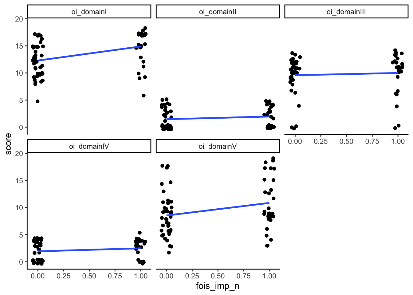
Logistic regressions
foisdomain_logr <- glm(fois_imp_n ~ oi_domainI + oi_domainII + oi_domainIII + oi_domainIV + oi_domainV, family = "binomial", data = analysis_included_lastexam)

foisdomain_logr %>%
  tidy() %>%
kable(digits = 3)| term | estimate | std.error | statistic | p.value |
|---|---|---|---|---|
| (Intercept) | -4.312 | 1.587 | -2.718 | 0.007 |
| oi_domainI | 0.261 | 0.105 | 2.493 | 0.013 |
| oi_domainII | -0.141 | 0.206 | -0.685 | 0.494 |
| oi_domainIII | -0.089 | 0.109 | -0.815 | 0.415 |
| oi_domainIV | 0.209 | 0.207 | 1.013 | 0.311 |
| oi_domainV | 0.098 | 0.082 | 1.194 | 0.233 |
Domain I is the only one significantly related to whether secretions would be impaired versus not. You can interpret the coefficient by taking the exponent of the estimate, 0.1845978, which is 1.2027347.
Respiratory Support
Point-biserial associations (note: treats domain scores as continuous):
analysis_included_lastexam %>%
  select(resp_imp_n, contains("domain")) %>%
  pivot_longer(cols = contains("domain"),
               names_to = "domain",
               values_to = "score") %>%
  group_by(domain) %>%
  summarize(pb_correlation = cor(resp_imp_n, score, use="pairwise.complete.obs"),
            n = sum(!is.na(score)),
            p = cor.test(resp_imp_n, score)$p.value) %>%
kable(digits = 2)| domain | pb_correlation | n | p |
|---|---|---|---|
| oi_domainI | 0.36 | 69 | 0.00 |
| oi_domainII | 0.23 | 69 | 0.06 |
| oi_domainIII | 0.07 | 68 | 0.59 |
| oi_domainIV | 0.03 | 68 | 0.78 |
| oi_domainV | 0.37 | 69 | 0.00 |
Plots:
analysis_included_lastexam %>%
  select(resp_imp_n, contains("domain")) %>%
  pivot_longer(cols = contains("domain"),
               names_to = "domain",
               values_to = "score") %>%
  ggplot(aes(x = resp_imp_n, y = score)) +
    geom_point(position = position_jitter(width = .05)) +
    geom_smooth(method = "lm", se = F) +
    facet_wrap(~domain) +
    theme_classic()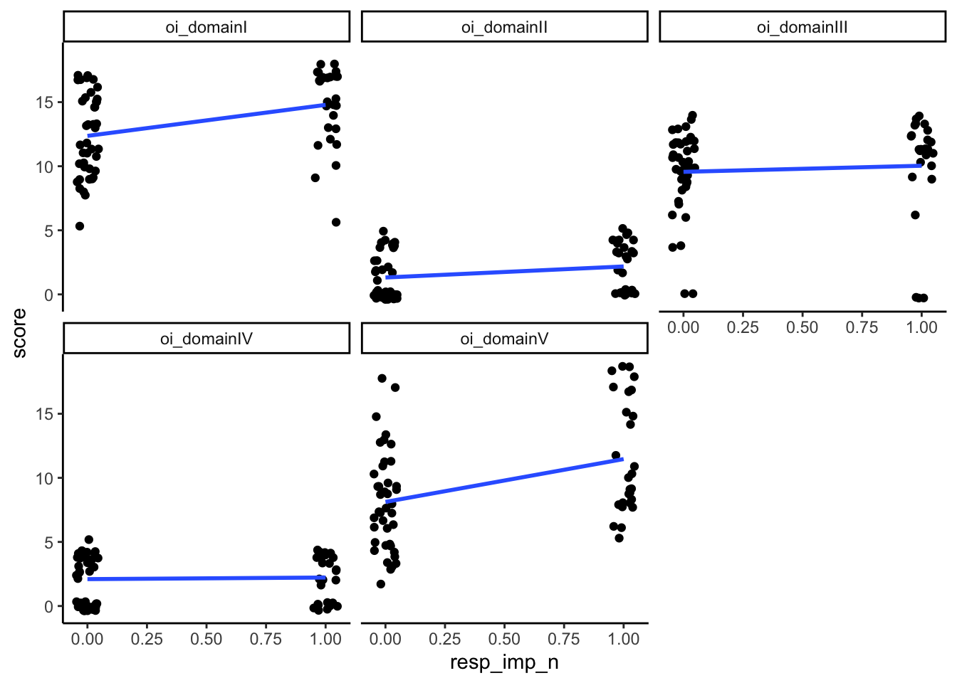
Logistic regressions
respdomain_logr <- glm(resp_imp_n ~ oi_domainI + oi_domainII + oi_domainIII + oi_domainIV + oi_domainV, family = "binomial", data = analysis_included_lastexam)

respdomain_logr %>%
  tidy() %>%
kable(digits = 3)| term | estimate | std.error | statistic | p.value |
|---|---|---|---|---|
| (Intercept) | -3.669 | 1.557 | -2.357 | 0.018 |
| oi_domainI | 0.177 | 0.102 | 1.739 | 0.082 |
| oi_domainII | 0.109 | 0.214 | 0.508 | 0.611 |
| oi_domainIII | -0.077 | 0.109 | -0.708 | 0.479 |
| oi_domainIV | -0.168 | 0.228 | -0.737 | 0.461 |
| oi_domainV | 0.183 | 0.089 | 2.044 | 0.041 |
None significantly predict having impaired respiration.
Which other components predict function?
For these, will look at phi coefficients as a measure of association between impairment in specific components and impairments in functioning. Phi can be interpreted similarly to correlation coefficients, although it measures association between two binary variables. We can use a chi-squared test to assess whether the two variables are associated.
See the Kinematics analysis for these analyses for PCR Mean for last exam
TBR (OI17)
Secreation management
analysis_included_lastexam %>%
  filter(!is.na(oi_17_imp)) %>%
  group_by(oi_17_imp, sec_imp) %>%
  tally() %>%
  pivot_wider(names_from = sec_imp,
              values_from = n) %>%
kable()| oi_17_imp | No | Yes, suctioning needed |
|---|---|---|
| No | 38 | 11 |
| Yes | 11 | 9 |
table_oi17_sec <- table(analysis_included_lastexam$oi_17_imp_n, analysis_included_lastexam$sec_imp_n)

phi(table_oi17_sec)
[1] 0.23chisq.test(table_oi17_sec)
    Pearson's Chi-squared test with Yates' continuity correction

data:  table_oi17_sec
X-squared = 2.4989, df = 1, p-value = 0.1139
FOIS
analysis_included_lastexam %>%
  filter(!is.na(oi_17_imp)) %>%
  group_by(oi_17_imp, fois_imp) %>%
  tally() %>%
  pivot_wider(names_from = fois_imp,
              values_from = n) %>%
kable()| oi_17_imp | No | Yes |
|---|---|---|
| No | 29 | 20 |
| Yes | 12 | 8 |
table_oi17_fois <- table(analysis_included_lastexam$oi_17_imp_n, analysis_included_lastexam$fois_imp_n)

phi(table_oi17_fois)
[1] -0.01chisq.test(table_oi17_fois)
    Pearson's Chi-squared test with Yates' continuity correction

data:  table_oi17_fois
X-squared = 0, df = 1, p-value = 1
Respiratory support
analysis_included_lastexam %>%
  filter(!is.na(oi_17_imp)) %>%
  group_by(oi_17_imp, resp_text_any) %>%
  tally() %>%
  pivot_wider(names_from = resp_text_any,
              values_from = n) %>%
kable()| oi_17_imp | BiPAP or Ventilator | None |
|---|---|---|
| No | 16 | 33 |
| Yes | 12 | 8 |
table_oi17_resp <- table(analysis_included_lastexam$oi_17_imp_n, analysis_included_lastexam$resp_imp_n)

phi(table_oi17_resp)
[1] 0.25chisq.test(table_oi17_resp)
    Pearson's Chi-squared test with Yates' continuity correction

data:  table_oi17_resp
X-squared = 3.3439, df = 1, p-value = 0.06745
PSS (OI 18)
Secreation management
analysis_included_lastexam %>%
  filter(!is.na(oi_18_imp)) %>%
  group_by(oi_18_imp, sec_imp) %>%
  tally() %>%
  pivot_wider(names_from = sec_imp,
              values_from = n) %>%
kable()| oi_18_imp | No | Yes, suctioning needed |
|---|---|---|
| No | 46 | 12 |
| Yes | 3 | 8 |
table_oi18_sec <- table(analysis_included_lastexam$oi_18_imp_n, analysis_included_lastexam$sec_imp_n)

phi(table_oi18_sec)
[1] 0.42chisq.test(table_oi18_sec) #small expected counts, will use fisher's exact test
    Pearson's Chi-squared test with Yates' continuity correction

data:  table_oi18_sec
X-squared = 9.7673, df = 1, p-value = 0.001776
fisher.test(table_oi18_sec)
    Fisher's Exact Test for Count Data

data:  table_oi18_sec
p-value = 0.001386
alternative hypothesis: true odds ratio is not equal to 1
95 percent confidence interval:
  1.979133 66.159149
sample estimates:
odds ratio
  9.778574
FOIS
analysis_included_lastexam %>%
  filter(!is.na(oi_18_imp)) %>%
  group_by(oi_18_imp, fois_imp) %>%
  tally() %>%
  pivot_wider(names_from = fois_imp,
              values_from = n) %>%
kable()| oi_18_imp | No | Yes |
|---|---|---|
| No | 38 | 20 |
| Yes | 3 | 8 |
table_oi18_fois <- table(analysis_included_lastexam$oi_18_imp_n, analysis_included_lastexam$fois_imp_n)

phi(table_oi18_fois)
[1] 0.29chisq.test(table_oi18_fois) #small expected counts, will use fishers
    Pearson's Chi-squared test with Yates' continuity correction

data:  table_oi18_fois
X-squared = 4.1348, df = 1, p-value = 0.04201
fisher.test(table_oi18_fois)
    Fisher's Exact Test for Count Data

data:  table_oi18_fois
p-value = 0.04052
alternative hypothesis: true odds ratio is not equal to 1
95 percent confidence interval:
  1.04096 32.12429
sample estimates:
odds ratio
  4.941883
Respiratory support
analysis_included_lastexam %>%
  filter(!is.na(oi_18_imp)) %>%
  group_by(oi_18_imp, resp_text_any) %>%
  tally() %>%
  pivot_wider(names_from = resp_text_any,
              values_from = n) %>%
kable()| oi_18_imp | BiPAP or Ventilator | None |
|---|---|---|
| No | 20 | 38 |
| Yes | 8 | 3 |
table_oi18_resp <- table(analysis_included_lastexam$oi_18_imp_n, analysis_included_lastexam$resp_imp_n)

phi(table_oi18_resp)
[1] 0.29chisq.test(table_oi18_resp) #small expected counts, will use fisher's
    Pearson's Chi-squared test with Yates' continuity correction

data:  table_oi18_resp
X-squared = 4.1348, df = 1, p-value = 0.04201
fisher.test(table_oi18_resp)
    Fisher's Exact Test for Count Data

data:  table_oi18_resp
p-value = 0.04052
alternative hypothesis: true odds ratio is not equal to 1
95 percent confidence interval:
  1.04096 32.12429
sample estimates:
odds ratio
  4.941883
Compile and Export components of presymptomatic group
presymp_chart <- chartreview_included %>%
  filter(treat_group == "Before Symptoms") %>%
  select(studyid, smn2, screenc, sympoms, treatment_age, starts_with("age_mbs"), starts_with("fois_cur_mbs"))

presymp_ois <- analysis_included_last_b %>%
  select(Subject.ID, oi_7, oi_17, oi_19, oi_20, oi_21)

#combine
presymp <- presymp_chart %>%
  full_join(presymp_ois, by = c("studyid" = "Subject.ID"))

#export
#write.csv(presymp, file = "../data/SMA_PreSymptomatic_Treated_Table.csv", row.names = F)
Save out files for other analyses
# #write out data files for included participants
# save(analysis_included, analysis_included_lastexam, chartreview_included, file = "../data/SMA_analysis_files.Rdata")
Session Information
sessionInfo()R version 4.5.1 (2025-06-13)
Platform: x86_64-apple-darwin20
Running under: macOS Sonoma 14.4.1
Matrix products: default
BLAS: /Library/Frameworks/R.framework/Versions/4.5-x86_64/Resources/lib/libRblas.0.dylib
LAPACK: /Library/Frameworks/R.framework/Versions/4.5-x86_64/Resources/lib/libRlapack.dylib; LAPACK version 3.12.1
locale:
[1] en_US.UTF-8/en_US.UTF-8/en_US.UTF-8/C/en_US.UTF-8/en_US.UTF-8
time zone: America/Chicago
tzcode source: internal
attached base packages:
[1] grid stats graphics grDevices utils datasets methods
[8] base
other attached packages:
[1] psych_2.5.6 broom_1.0.8 effectsize_1.0.1 effsize_0.8.1
[5] nptest_1.1 lme4_1.1-37 Matrix_1.7-3 purrr_1.0.4
[9] pander_0.6.6 knitr_1.50 vcd_1.4-13 readxl_1.4.5
[13] tidyr_1.3.1 ggplot2_3.5.2 dplyr_1.1.4
loaded via a namespace (and not attached):
[1] gtable_0.3.6 xfun_0.52 bslib_0.9.0 bayestestR_0.16.1
[5] insight_1.3.1 lattice_0.22-7 vctrs_0.6.5 tools_4.5.1
[9] Rdpack_2.6.4 generics_0.1.4 parallel_4.5.1 datawizard_1.1.0
[13] tibble_3.3.0 pacman_0.5.1 pkgconfig_2.0.3 RColorBrewer_1.1-3
[17] lifecycle_1.0.4 compiler_4.5.1 farver_2.1.2 mnormt_2.1.1
[21] htmltools_0.5.8.1 sass_0.4.10 yaml_2.3.10 pillar_1.10.2
[25] nloptr_2.2.1 jquerylib_0.1.4 MASS_7.3-65 cachem_1.1.0
[29] reformulas_0.4.1 boot_1.3-31 nlme_3.1-168 tidyselect_1.2.1
[33] digest_0.6.37 mvtnorm_1.3-3 labeling_0.4.3 splines_4.5.1
[37] fastmap_1.2.0 colorspace_2.1-1 cli_3.6.5 magrittr_2.0.3
[41] withr_3.0.2 scales_1.4.0 backports_1.5.0 estimability_1.5.1
[45] rmarkdown_2.29 emmeans_1.11.1 cellranger_1.1.0 zoo_1.8-14
[49] coda_0.19-4.1 evaluate_1.0.4 parameters_0.27.0 rbibutils_2.3
[53] lmtest_0.9-40 mgcv_1.9-3 rlang_1.1.6 Rcpp_1.0.14
[57] xtable_1.8-4 glue_1.8.0 rstudioapi_0.17.1 minqa_1.2.8
[61] jsonlite_2.0.0 R6_2.6.1