Read in the data

## load in required data 
SMA_DAT <- read.csv("~/Library/CloudStorage/Box-Box/CLA RSS Data Sharing/1022295_McGrattan_SMA_KINEMATICS/SMA_Data/SMA_DAT_summary_last20250811.csv", header = T)
SMA_DAT_full <- read.csv("~/Library/CloudStorage/Box-Box/CLA RSS Data Sharing/1022295_McGrattan_SMA_KINEMATICS/SMA_Data/SMA_DAT_combined_last20250811.csv")

#load in included and last exam data 
load("~/Library/CloudStorage/Box-Box/CLA RSS Data Sharing/577565_McGrattan_SMA/BABYVFSSIMP/data/SMA_analysis_files.Rdata")

#Participants NZ_01 and PRI_O4 only have one observation/swallow, so removing them from the analysis; also remove those who are not on inclusion list. Also remove untreated group
SMA_DAT <- SMA_DAT %>% 
  filter(!(Subject.ID %in% c("NZ_01", "PRI_04"))) %>% 
  filter(!is.na(treat_group))

SMA_DAT_full <- SMA_DAT_full %>% 
  filter(!(Subject.ID %in% c("NZ_01", "PRI_04"))) %>% 
  filter(!is.na(treat_group))

#add in Secretion, Respiration, and FOIS impairments into the data
funct_impair <- analysis_included_lastexam %>% 
  select(Subject.ID, fois_imp, fois_imp_n, resp_text_any, resp_imp_n, sec_imp, sec_imp_n)

Who is missing from the kinematics data?

analysis_included_lastexam %>% 
  filter(Subject.ID %in% SMA_DAT$Subject.ID == FALSE) %>% 
  select(Subject.ID, studyid_clean, treat_group) %>% 
  kable()


SMA_DAT <- SMA_DAT %>% 
  inner_join(funct_impair, by="Subject.ID")

Total Sample N

For the BABYVFSSIMP, there were two analyses - one for untreated participants and the other comparing groups who were treated before vs after symptoms appeared. This analysis just looks at the treated before vs after symptoms. This uses data from the last exam.

## number of infants in treated and untreated groups

visit_summary <- SMA_DAT %>% 
  filter(!is.na(treat_group)) %>% 
  group_by(treat_group) %>% 
  summarize(avg_obs = mean(n_obvs), 
            min_obs = min(n_obvs), 
            max_obs = max(n_obvs), 
            N = n_distinct(Subject.ID))

visit_summary %>% 
  kable(col.names = c("Treated", "Average Swallows", "Min Swallows", "Max Swallows", "N individuals"), 
        digits = 2)

Treated	Average Swallows	Min Swallows	Max Swallows	N individuals
After Symptoms	23.39	1	127	51
Before Symptoms	24.67	2	61	17

PCR cleaning

Who in Before has PCR >= 0.5?

Any swallow:

SMA_DAT_full %>% 
  filter(Measurement_name == "PCR", value >= 0.5, treat_group == "Before Symptoms") %>% 
  select(Subject.ID, Participant_Num, Swallow_Number, Measurement_name, value) %>% 
  arrange(Subject.ID, Participant_Num, Swallow_Number) %>% 
  kable()

Worst/best/mean:

SMA_DAT %>% 
  filter(Measurement_name == "PCR", treat_group == "Before Symptoms") %>%
  filter(Mean >= 0.5 | Worst_OI >= 0.5 | Best_OI >= 0.5) %>% 
  select(Subject.ID,  Measurement_name, Mean, Worst_OI, Best_OI) %>% 
  arrange(Subject.ID) %>% 
  kable()

Align OI scores for OI_17 (tongue base), OI_19 , and OI_20 (residue) with worst PCR scores.

pcrworst <- SMA_DAT %>% 
  filter(Measurement_name == "PCR") %>% 
  select(Subject.ID, Worst_OI, treat_group) %>% 
  rename(PCR_Worst_OI = Worst_OI)

analysis_included_lastexam %>% 
  select(Subject.ID, oi_17, oi_19, oi_20) %>% 
  right_join(pcrworst, by="Subject.ID") %>% 
  relocate(treat_group, .after = Subject.ID) %>% 
  arrange(treat_group, PCR_Worst_OI) %>% 
  kable()

Descriptive Statistics

Overall descriptives

First, take averages across all swallows in each participants.

SMA_DAT_summary_indiv <- SMA_DAT_full %>% 
  group_by(Measurement_name, treat_group, Subject.ID) %>% 
  summarize(Mean = mean(value, na.rm=T), 
            SD = sd(value, na.rm=T), 
            N = n())

datatable(SMA_DAT_summary_indiv, options = list(pageLength = 10))

Then take the mean and SD of these means

SMA_DAT_summary_indiv %>% 
  group_by(Measurement_name, treat_group) %>% 
  summarize(Overall_Mean = mean(Mean, na.rm=T), 
            Overall_SD = sd(Mean, na.rm=T), 
            N = n()) %>% 
  kbl(digits=2) %>% 
  kable_styling()

Measurement_name	treat_group	Overall_Mean	Overall_SD	N
HPT	After Symptoms	1.01	0.99	51
HPT	Before Symptoms	0.76	0.74	17
OPT	After Symptoms	0.78	0.62	51
OPT	Before Symptoms	0.95	1.18	17
PCR	After Symptoms	0.15	0.16	51
PCR	Before Symptoms	0.03	0.02	17
PESop	After Symptoms	0.24	0.09	51
PESop	Before Symptoms	0.22	0.06	17
TPT	After Symptoms	1.74	1.40	51
TPT	Before Symptoms	1.72	1.87	17

Visualizations

SMA_DAT_l <- SMA_DAT %>% 
  select(Subject.ID,treat_group, Measurement_name, Worst_OI, Best_OI, Mean) %>% 
  pivot_longer(cols = Worst_OI:Mean, 
               names_to = "Statistic", 
               values_to = "Value")


SMA_DAT_l %>% 
  filter(Statistic == "Mean") %>% 
  ggplot(aes(x = treat_group, y=Value)) +
  geom_boxplot() +
  facet_wrap(~Measurement_name, scales = "free") +
  labs(title = "Mean") +
  theme_classic() +
  theme(axis.text.x = element_text(angle = 90))

## Warning: Removed 14 rows containing non-finite outside the scale range
## (`stat_boxplot()`).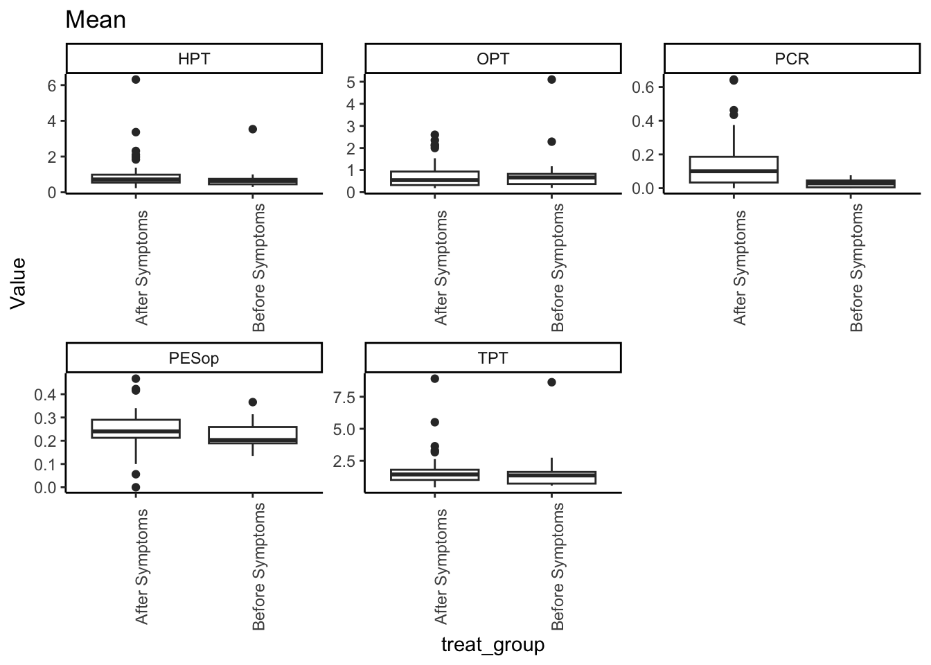

Do OI scores differ for by treatment?

These are continuous measures, although groups are slightly unbalanced in terms of numbers. Will use parametric comparisons for now. t-tests will be used to asses differences between means for each measure.

PCR - Asymp vs Symp

PCR - Mean Score

Means and SD

SMA_DAT %>% 
  filter(Measurement_name == "PCR") %>% 
 group_by(treat_group) %>% 
    summarize(Average = mean(Mean, na.rm=T), 
            SD = sd(Mean, na.rm=T), 
            N = sum(!is.na(Mean))) %>% 
  kable(digits=2)

treat_group	Average	SD	N
After Symptoms	0.15	0.16	49
Before Symptoms	0.03	0.02	17

#look at the raw distributions
SMA_DAT %>% 
  filter(Measurement_name == "PCR") %>% 
  ggplot(aes(x = treat_group, y=Mean)) +
  geom_boxplot() +
  theme_classic()

## Warning: Removed 2 rows containing non-finite outside the scale range
## (`stat_boxplot()`).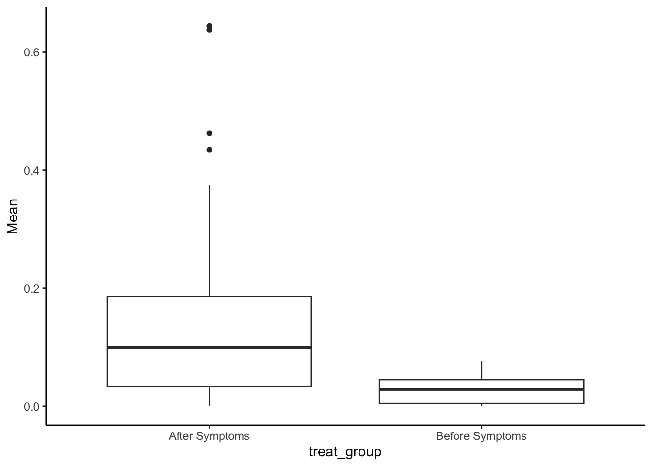

#t.test
(pcr_m <- t.test(Mean ~ treat_group, data = filter(SMA_DAT, Measurement_name == "PCR")))

## 
##  Welch Two Sample t-test
## 
## data:  Mean by treat_group
## t = 5.1029, df = 53.801, p-value = 4.48e-06
## alternative hypothesis: true difference in means between group After Symptoms and group Before Symptoms is not equal to 0
## 95 percent confidence interval:
##  0.07121631 0.16340334
## sample estimates:
##  mean in group After Symptoms mean in group Before Symptoms 
##                    0.14582697                    0.02851715

#cohen's d for effect size
cohen.d(Mean ~ treat_group, data = filter(SMA_DAT, Measurement_name == "PCR"))

## Call: cohen.d(x = Mean ~ treat_group, data = filter(SMA_DAT, Measurement_name == 
##     "PCR"))
## Cohen d statistic of difference between two means
##      lower effect upper
## Mean -1.45  -0.88  -0.3
## 
## Multivariate (Mahalanobis) distance between groups
## [1] 0.88
## r equivalent of difference between two means
##  Mean 
## -0.36

Dichotimized PCR score

Could you dichotomize average PCR for each kid into <0.2 and >0.2 (profound impairment), give N% for the kids with each in pre and post symptomatic groups, and compare those proportions between groups?

pcr_group <- SMA_DAT %>% 
  filter(Measurement_name == "PCR") %>% 
  mutate(pcrimp = ifelse(Mean <= 0.2, "No", "Yes"))

pcr_group %>% 
  filter(!is.na(pcrimp)) %>% 
  group_by(treat_group, pcrimp) %>% 
  tally() %>% 
  group_by(treat_group) %>% 
  mutate(percent = n/sum(n)*100) %>% 
  kable(digits = 1)

treat_group	pcrimp	n	percent
After Symptoms	No	37	75.5
After Symptoms	Yes	12	24.5
Before Symptoms	No	17	100.0

pcrimptab <- table( pcr_group$pcrimp, pcr_group$treat_group)

fisher.test(pcrimptab)

## 
##  Fisher's Exact Test for Count Data
## 
## data:  pcrimptab
## p-value = 0.02742
## alternative hypothesis: true odds ratio is not equal to 1
## 95 percent confidence interval:
##  0.0000000 0.9084527
## sample estimates:
## odds ratio 
##          0

PESop - Asymp vs Symp

PESop - Mean Score

Means and SD

SMA_DAT %>% 
  filter(Measurement_name == "PESop") %>% 
 group_by(treat_group) %>% 
    summarize(Average = mean(Mean, na.rm=T), 
            SD = sd(Mean, na.rm=T), 
            N = sum(!is.na(Mean))) %>% 
  kable(digits=2)

treat_group	Average	SD	N
After Symptoms	0.24	0.09	48
Before Symptoms	0.22	0.06	17

#look at the raw distributions
SMA_DAT %>% 
  filter(Measurement_name == "PESop") %>% 
  ggplot(aes(x = treat_group, y=Mean)) +
  geom_boxplot() +
  theme_classic()

## Warning: Removed 3 rows containing non-finite outside the scale range
## (`stat_boxplot()`).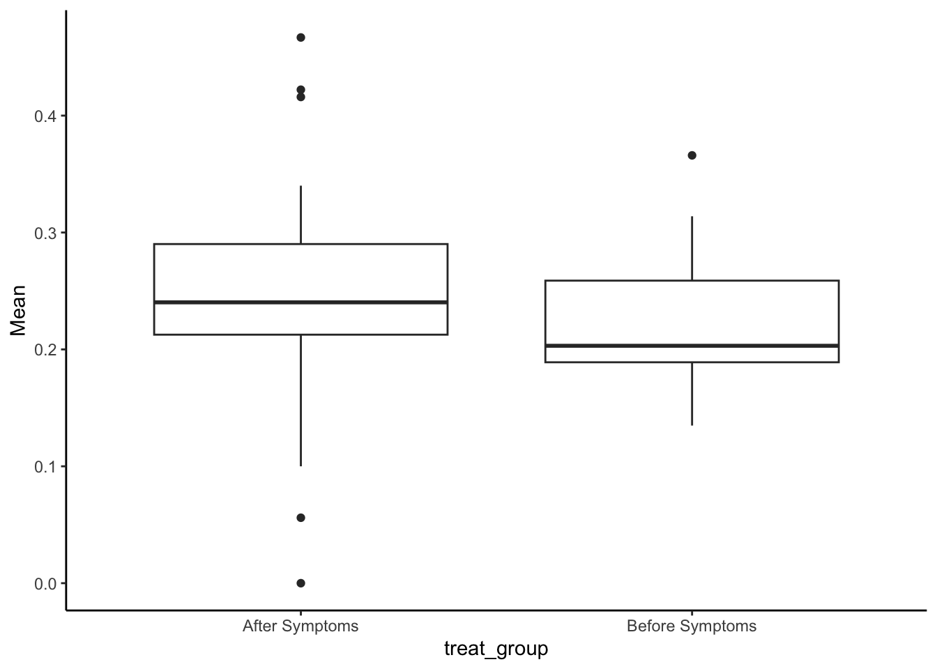

#t.test
(pesop_m <- t.test(Mean ~ treat_group, data = filter(SMA_DAT, Measurement_name == "PESop")))

## 
##  Welch Two Sample t-test
## 
## data:  Mean by treat_group
## t = 0.84042, df = 40.039, p-value = 0.4057
## alternative hypothesis: true difference in means between group After Symptoms and group Before Symptoms is not equal to 0
## 95 percent confidence interval:
##  -0.02343201  0.05679291
## sample estimates:
##  mean in group After Symptoms mean in group Before Symptoms 
##                     0.2399721                     0.2232917

#cohen's d
cohen.d(Mean ~ treat_group, data = filter(SMA_DAT, Measurement_name == "PESop"))

## Call: cohen.d(x = Mean ~ treat_group, data = filter(SMA_DAT, Measurement_name == 
##     "PESop"))
## Cohen d statistic of difference between two means
##      lower effect upper
## Mean -0.76   -0.2  0.35
## 
## Multivariate (Mahalanobis) distance between groups
## [1] 0.2
## r equivalent of difference between two means
##  Mean 
## -0.09

Does PCR scores predict functional impairments?

Using analyses similar to the Babyvfssimp scores. Look at point-biserial correlations and logistic regression.

Secreation management

Point-biserial associations :

SMA_DAT %>% 
  filter(Measurement_name == "PCR") %>% 
  select(sec_imp_n, Mean) %>% 
  summarize(mean_corr = cor(sec_imp_n, Mean, use="pairwise.complete.obs"), 
            n = sum(!is.na(Mean)), 
            p = cor.test(sec_imp_n, Mean)$p.value) %>% 
  kable(digits = 2)

mean_corr	n	p
0.26	66	0.03

Plots:

SMA_DAT %>%
  filter(Measurement_name == "PCR") %>% 
  ggplot(aes(x = sec_imp_n, y = Mean)) +
    geom_point(position = position_jitter(width = .05)) +
    geom_smooth(method = "lm", se = F) +
    theme_classic()

## Warning: Removed 2 rows containing non-finite outside the scale range
## (`stat_smooth()`).

## Warning: Removed 2 rows containing missing values or values outside
## the scale range (`geom_point()`).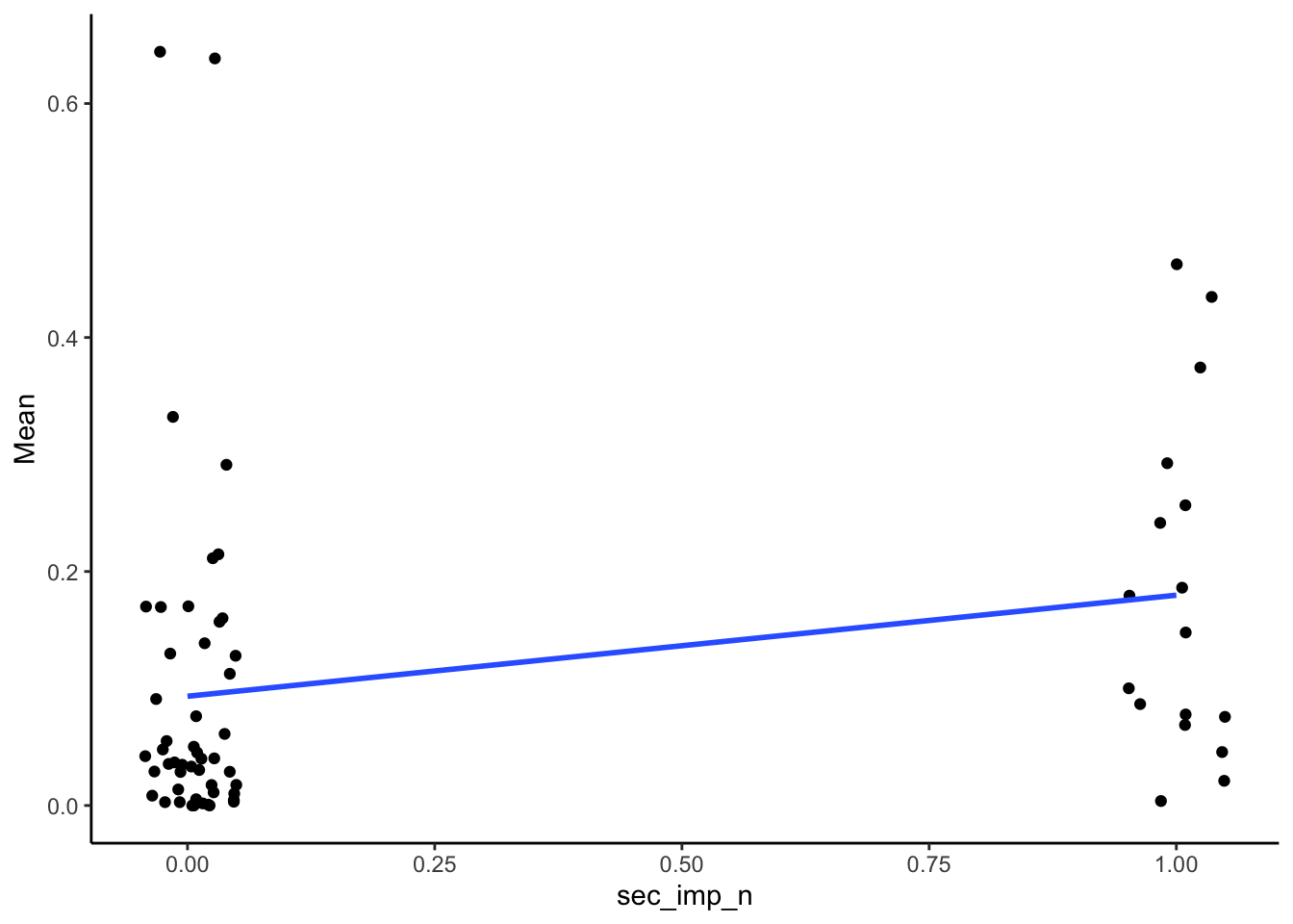

Logistic regressions

secpcr_logr <- glm(sec_imp_n ~ Mean, family = "binomial", data = filter(SMA_DAT, Measurement_name == "PCR"))

secpcr_logr %>% 
  tidy() %>% 
  kable(digits = 3)

term	estimate	std.error	statistic	p.value
(Intercept)	-1.551	0.393	-3.949	0.000
Mean	3.799	1.916	1.983	0.047

summary(secpcr_logr)

## 
## Call:
## glm(formula = sec_imp_n ~ Mean, family = "binomial", data = filter(SMA_DAT, 
##     Measurement_name == "PCR"))
## 
## Coefficients:
##             Estimate Std. Error z value Pr(>|z|)    
## (Intercept)  -1.5508     0.3927  -3.949 7.84e-05 ***
## Mean          3.7988     1.9161   1.983   0.0474 *  
## ---
## Signif. codes:  0 '***' 0.001 '**' 0.01 '*' 0.05 '.' 0.1 ' ' 1
## 
## (Dispersion parameter for binomial family taken to be 1)
## 
##     Null deviance: 75.307  on 65  degrees of freedom
## Residual deviance: 71.131  on 64  degrees of freedom
##   (2 observations deleted due to missingness)
## AIC: 75.131
## 
## Number of Fisher Scoring iterations: 4

Mean PCR significant predicts impairment in secretion management. 3.7987782, the increase in odds for every 1 point increase in PCR (which note the small scale of this value) is 44.6466026

FOIS

Point-biserial associations

SMA_DAT %>% 
  filter(Measurement_name == "PCR") %>% 
  summarize(pb_correlation = cor(fois_imp_n, Mean, use="pairwise.complete.obs"), 
            n = sum(!is.na(Mean)), 
            p = cor.test(fois_imp_n, Mean)$p.value) %>% 
  kable(digits = 2)

pb_correlation	n	p
0.15	66	0.23

Plots:

SMA_DAT %>% 
  filter(Measurement_name == "PCR") %>% 
  ggplot(aes(x = fois_imp_n, y = Mean)) +
    geom_point(position = position_jitter(width = .05)) +
    geom_smooth(method = "lm", se = F) +
    theme_classic()

## Warning: Removed 2 rows containing non-finite outside the scale range
## (`stat_smooth()`).

## Warning: Removed 2 rows containing missing values or values outside
## the scale range (`geom_point()`).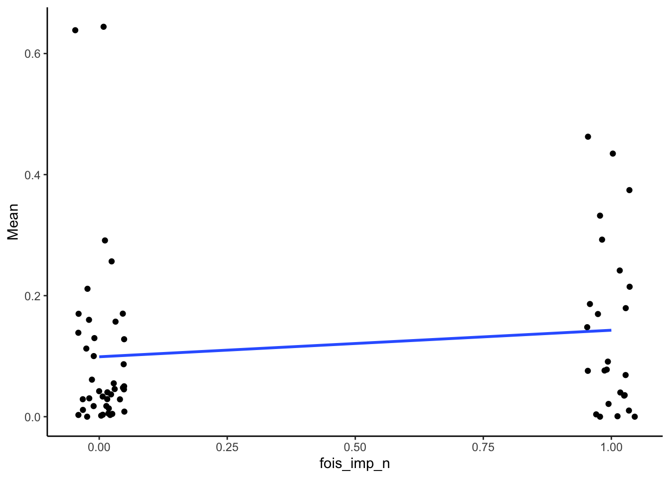

Logistic regressions

foispcr_logr <- glm(fois_imp_n ~ Mean, family = "binomial", data = filter(SMA_DAT, Measurement_name == "PCR"))

foispcr_logr %>% 
  tidy() %>% 
  kable(digits = 3)

term	estimate	std.error	statistic	p.value
(Intercept)	-0.744	0.334	-2.228	0.026
Mean	2.101	1.782	1.179	0.238

Respiratory Support

Point-biserial associations

SMA_DAT %>% 
  filter(Measurement_name == "PCR") %>% 
  summarize(pb_correlation = cor(resp_imp_n, Mean, use="pairwise.complete.obs"), 
            n = sum(!is.na(Mean)), 
            p = cor.test(resp_imp_n, Mean)$p.value) %>% 
  kable(digits = 2)

pb_correlation	n	p
0.32	66	0.01

Plots:

SMA_DAT %>% 
  filter(Measurement_name == "PCR") %>% 
  ggplot(aes(x = resp_imp_n, y = Mean)) +
    geom_point(position = position_jitter(width = .05)) +
    geom_smooth(method = "lm", se = F) +
    theme_classic()

## Warning: Removed 2 rows containing non-finite outside the scale range
## (`stat_smooth()`).

## Warning: Removed 2 rows containing missing values or values outside
## the scale range (`geom_point()`).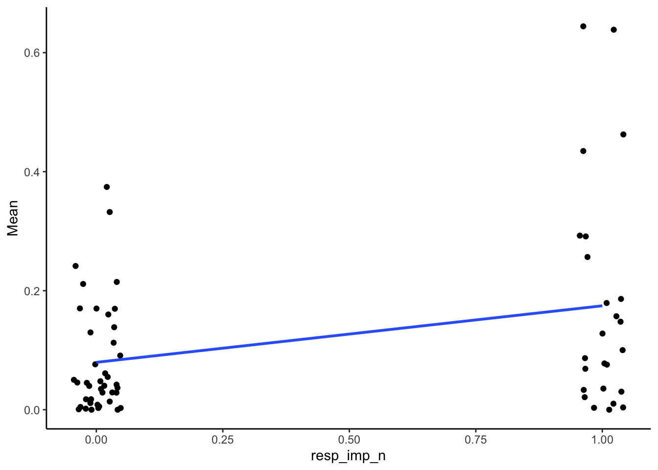

Logistic regressions

resppcr_logr <- glm(resp_imp_n ~ Mean, family = "binomial", data = filter(SMA_DAT, Measurement_name == "PCR"))

resppcr_logr %>% 
  tidy() %>% 
  kable(digits = 3)

term	estimate	std.error	statistic	p.value
(Intercept)	-1.092	0.361	-3.022	0.003
Mean	5.086	2.170	2.344	0.019

Exponentiated effect = 161.6691562.

Comparing PCR and Domain V predictions of Secretion impairment

Putting the datasets together

analysis_included_lastexam_domains <- analysis_included_lastexam %>% 
  select(Subject.ID, contains("domain"))


SMA_VFSS_combo <- SMA_DAT %>% 
  filter(Measurement_name == "PCR") %>% 
  inner_join(analysis_included_lastexam_domains, by="Subject.ID") %>% 
  filter(!is.na(Mean)) #remove two who have missing PCR data

Look at correlation between PCR and domain V

SMA_VFSS_combo %>% 
summarize(pb_correlation = cor(oi_domainV, Mean, use="pairwise.complete.obs"), 
            n = sum(!is.na(Mean)), 
            p = cor.test(oi_domainV, Mean)$p.value) %>% 
  kable(digits = 2)

pb_correlation	n	p
0.67	66	0

Very strongly correlated

SMA_VFSS_combo %>%
 ggplot(aes(x = oi_domainV, y = Mean)) +
    geom_point() +
    geom_smooth(method = "lm", se = F) +
    theme_classic()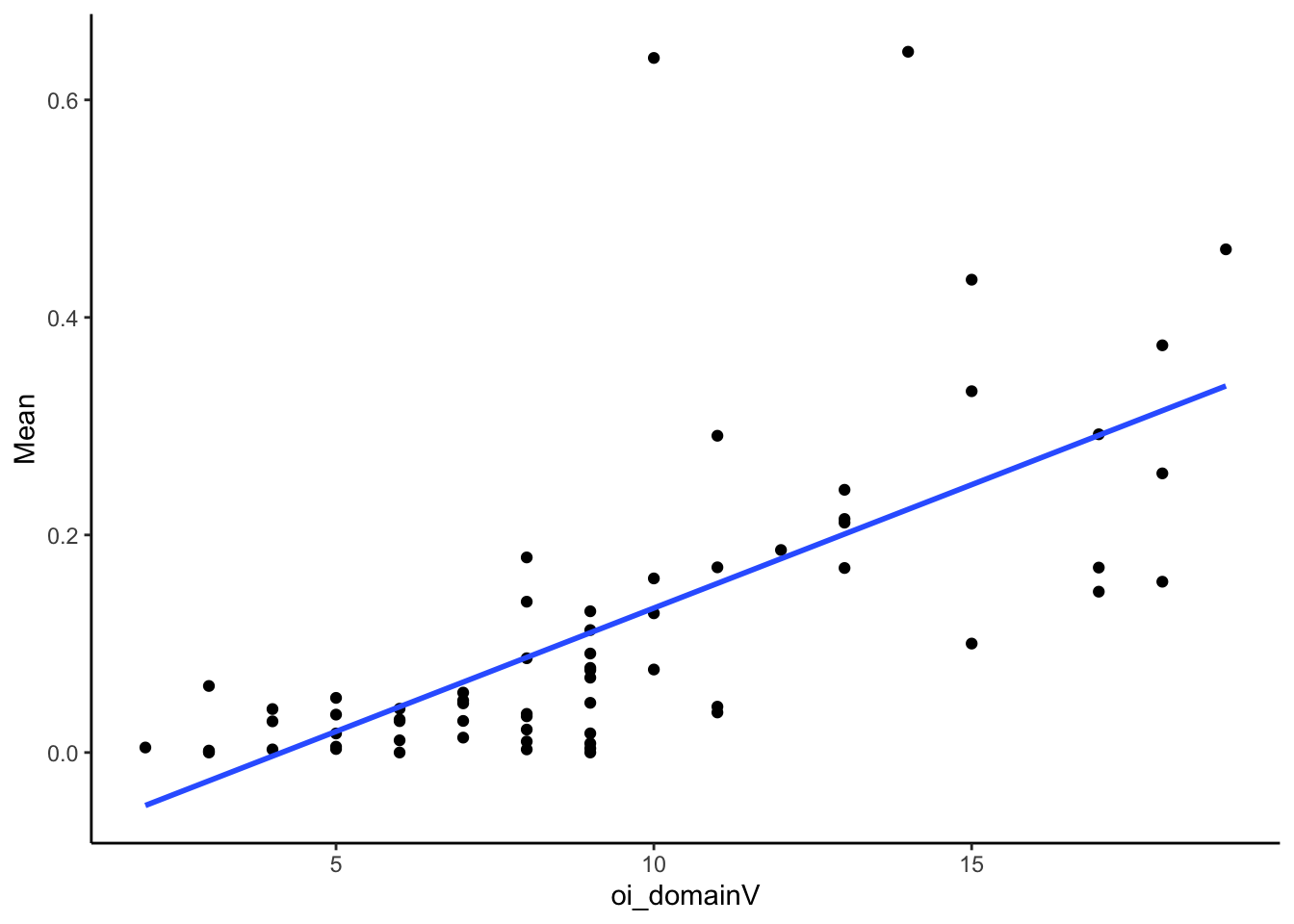

Included in model together? Likely to have multi-colinearity due to high correlation

#start with domain V only (reduced model)
m1_dv_first <- glm(sec_imp_n ~ oi_domainV, family = "binomial", data = SMA_VFSS_combo)

#then add PCR
m2_dv_first <-  glm(sec_imp_n ~ oi_domainV + Mean, family = "binomial", data = SMA_VFSS_combo)

#compare
anova(m1_dv_first, m2_dv_first)

## Analysis of Deviance Table
## 
## Model 1: sec_imp_n ~ oi_domainV
## Model 2: sec_imp_n ~ oi_domainV + Mean
##   Resid. Df Resid. Dev Df Deviance Pr(>Chi)
## 1        64     61.275                     
## 2        63     60.964  1  0.31117    0.577

AIC(m1_dv_first, m2_dv_first)

##             df      AIC
## m1_dv_first  2 65.27537
## m2_dv_first  3 66.96420

Very little difference between models…

Try the other order (entering Mean first to see if domain score adds more information)

#start with PCR only (reduced model)
m1_pcr_first <- glm(sec_imp_n ~ Mean, family = "binomial", data = SMA_VFSS_combo)

#then add domainV
m2_pcr_first <-  glm(sec_imp_n ~ Mean + oi_domainV, family = "binomial", data = SMA_VFSS_combo)

#compare
anova(m1_pcr_first, m2_pcr_first)

## Analysis of Deviance Table
## 
## Model 1: sec_imp_n ~ Mean
## Model 2: sec_imp_n ~ Mean + oi_domainV
##   Resid. Df Resid. Dev Df Deviance Pr(>Chi)   
## 1        64     71.131                        
## 2        63     60.964  1   10.167  0.00143 **
## ---
## Signif. codes:  0 '***' 0.001 '**' 0.01 '*' 0.05 '.' 0.1 ' ' 1

AIC(m1_pcr_first, m2_pcr_first)

##              df      AIC
## m1_pcr_first  2 75.13109
## m2_pcr_first  3 66.96420

Does PESop scores predict functional impairments?

Using analyses similar to the Babyvfssimp scores. Look at point-biserial correlations and logistic regression.

Secreation management

Point-biserial associations :

SMA_DAT %>% 
  filter(Measurement_name == "PESop") %>% 
  select(sec_imp_n, Mean) %>% 
  summarize(mean_corr = cor(sec_imp_n, Mean, use="pairwise.complete.obs"), 
            n = sum(!is.na(Mean)), 
            p = cor.test(sec_imp_n, Mean)$p.value) %>% 
  kable(digits = 2)

mean_corr	n	p
-0.14	65	0.26

Plots:

SMA_DAT %>%
  filter(Measurement_name == "PESop") %>% 
  ggplot(aes(x = sec_imp_n, y = Mean)) +
    geom_point(position = position_jitter(width = .05)) +
    geom_smooth(method = "lm", se = F) +
    theme_classic()

## Warning: Removed 3 rows containing non-finite outside the scale range
## (`stat_smooth()`).

## Warning: Removed 3 rows containing missing values or values outside
## the scale range (`geom_point()`).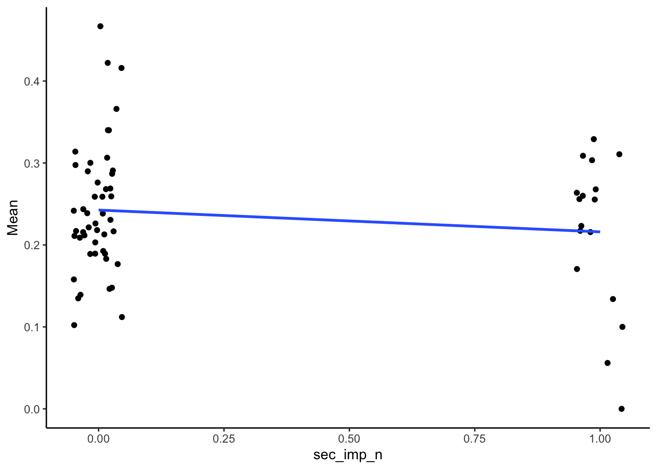

Logistic regressions

secpesop_logr <- glm(sec_imp_n ~ Mean, family = "binomial", data = filter(SMA_DAT, Measurement_name == "PESop"))

secpesop_logr %>% 
  tidy() %>% 
  kable(digits = 3)

term	estimate	std.error	statistic	p.value
(Intercept)	-0.105	0.849	-0.124	0.902
Mean	-4.069	3.582	-1.136	0.256

FOIS

Point-biserial associations

SMA_DAT %>% 
  filter(Measurement_name == "PESop") %>% 
  summarize(pb_correlation = cor(fois_imp_n, Mean, use="pairwise.complete.obs"), 
            n = sum(!is.na(Mean)), 
            p = cor.test(fois_imp_n, Mean)$p.value) %>% 
  kable(digits = 2)

pb_correlation	n	p
-0.04	65	0.76

Plots:

SMA_DAT %>% 
  filter(Measurement_name == "PESop") %>% 
  ggplot(aes(x = fois_imp_n, y = Mean)) +
    geom_point(position = position_jitter(width = .05)) +
    geom_smooth(method = "lm", se = F) +
    theme_classic()

## Warning: Removed 3 rows containing non-finite outside the scale range
## (`stat_smooth()`).

## Warning: Removed 3 rows containing missing values or values outside
## the scale range (`geom_point()`).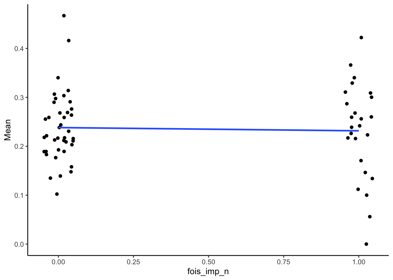

Logistic regressions

foispesop_logr <- glm(fois_imp_n ~ Mean, family = "binomial", data = filter(SMA_DAT, Measurement_name == "PESop"))

foispesop_logr %>% 
  tidy() %>% 
  kable(digits = 3)

term	estimate	std.error	statistic	p.value
(Intercept)	-0.238	0.774	-0.308	0.758
Mean	-0.986	3.123	-0.316	0.752

Respiratory Support

Point-biserial associations

SMA_DAT %>% 
  filter(Measurement_name == "PESop") %>% 
  summarize(pb_correlation = cor(resp_imp_n, Mean, use="pairwise.complete.obs"), 
            n = sum(!is.na(Mean)), 
            p = cor.test(resp_imp_n, Mean)$p.value) %>% 
  kable(digits = 2)

pb_correlation	n	p
0.04	65	0.73

Plots:

SMA_DAT %>% 
  filter(Measurement_name == "PESop") %>% 
  ggplot(aes(x = resp_imp_n, y = Mean)) +
    geom_point(position = position_jitter(width = .05)) +
    geom_smooth(method = "lm", se = F) +
    theme_classic()

## Warning: Removed 3 rows containing non-finite outside the scale range
## (`stat_smooth()`).

## Warning: Removed 3 rows containing missing values or values outside
## the scale range (`geom_point()`).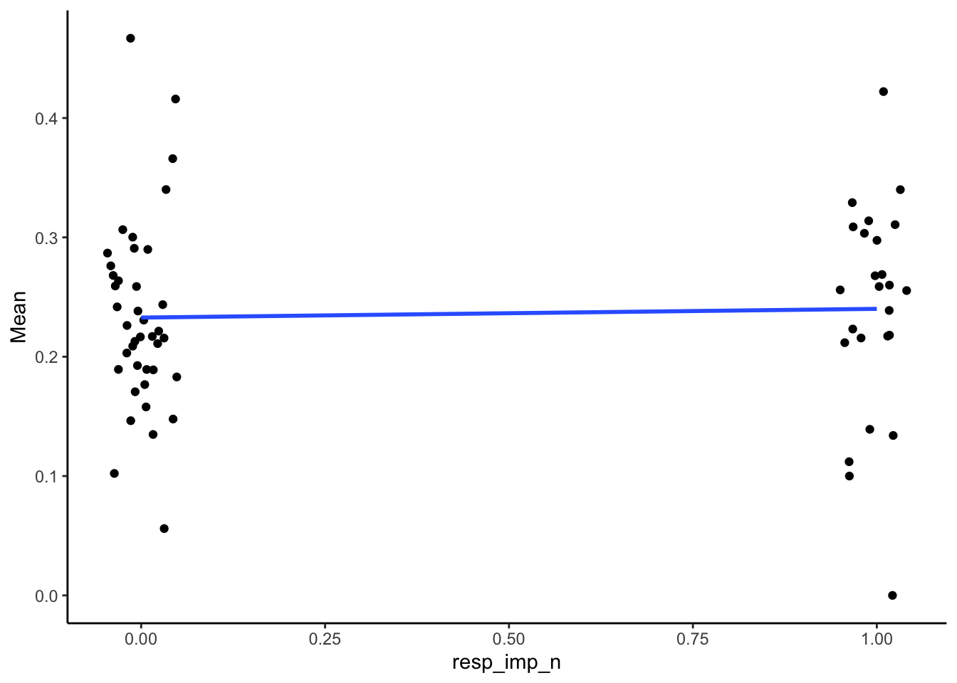

Logistic regressions

resppesop_logr <- glm(resp_imp_n ~ Mean, family = "binomial", data = filter(SMA_DAT, Measurement_name == "PESop"))

resppesop_logr %>% 
  tidy() %>% 
  kable(digits = 3)

term	estimate	std.error	statistic	p.value
(Intercept)	-0.728	0.784	-0.929	0.353
Mean	1.091	3.122	0.349	0.727

Session Information

sessionInfo()

## R version 4.5.1 (2025-06-13)
## Platform: x86_64-apple-darwin20
## Running under: macOS Sonoma 14.4.1
## 
## Matrix products: default
## BLAS:   /Library/Frameworks/R.framework/Versions/4.5-x86_64/Resources/lib/libRblas.0.dylib 
## LAPACK: /Library/Frameworks/R.framework/Versions/4.5-x86_64/Resources/lib/libRlapack.dylib;  LAPACK version 3.12.1
## 
## locale:
## [1] en_US.UTF-8/en_US.UTF-8/en_US.UTF-8/C/en_US.UTF-8/en_US.UTF-8
## 
## time zone: America/Chicago
## tzcode source: internal
## 
## attached base packages:
## [1] grid      stats     graphics  grDevices utils     datasets  methods  
## [8] base     
## 
## other attached packages:
##  [1] DT_0.33           kableExtra_1.4.0  psych_2.5.6       broom_1.0.8      
##  [5] effectsize_1.0.1  effsize_0.8.1     nptest_1.1        lme4_1.1-37      
##  [9] Matrix_1.7-3      irr_0.84.1        lpSolve_5.6.23    irrCAC_1.0       
## [13] purrr_1.0.4       pander_0.6.6      DescTools_0.99.60 knitr_1.50       
## [17] vcd_1.4-13        readxl_1.4.5      tidyr_1.3.1       ggplot2_3.5.2    
## [21] dplyr_1.1.4      
## 
## loaded via a namespace (and not attached):
##  [1] Rdpack_2.6.4       mnormt_2.1.1       gld_2.6.7          rlang_1.1.6       
##  [5] magrittr_2.0.3     e1071_1.7-16       compiler_4.5.1     mgcv_1.9-3        
##  [9] systemfonts_1.2.3  vctrs_0.6.5        stringr_1.5.1      pkgconfig_2.0.3   
## [13] fastmap_1.2.0      backports_1.5.0    labeling_0.4.3     utf8_1.2.6        
## [17] rmarkdown_2.29     tzdb_0.5.0         haven_2.5.5        nloptr_2.2.1      
## [21] xfun_0.52          cachem_1.1.0       jsonlite_2.0.0     parallel_4.5.1    
## [25] R6_2.6.1           bslib_0.9.0        stringi_1.8.7      RColorBrewer_1.1-3
## [29] boot_1.3-31        lmtest_0.9-40      jquerylib_0.1.4    cellranger_1.1.0  
## [33] estimability_1.5.1 Rcpp_1.0.14        zoo_1.8-14         parameters_0.27.0 
## [37] pacman_0.5.1       readr_2.1.5        splines_4.5.1      tidyselect_1.2.1  
## [41] rstudioapi_0.17.1  yaml_2.3.10        lattice_0.22-7     tibble_3.3.0      
## [45] withr_3.0.2        bayestestR_0.16.1  coda_0.19-4.1      evaluate_1.0.4    
## [49] proxy_0.4-27       xml2_1.3.8         pillar_1.10.2      reformulas_0.4.1  
## [53] insight_1.3.1      generics_0.1.4     hms_1.1.3          scales_1.4.0      
## [57] rootSolve_1.8.2.4  minqa_1.2.8        xtable_1.8-4       class_7.3-23      
## [61] glue_1.8.0         emmeans_1.11.1     lmom_3.2           tools_4.5.1       
## [65] data.table_1.17.6  forcats_1.0.0      Exact_3.3          fs_1.6.6          
## [69] mvtnorm_1.3-3      rbibutils_2.3      crosstalk_1.2.1    datawizard_1.1.0  
## [73] colorspace_2.1-1   nlme_3.1-168       cli_3.6.5          textshaping_1.0.1 
## [77] expm_1.0-0         viridisLite_0.4.2  svglite_2.2.1      gtable_0.3.6      
## [81] sass_0.4.10        digest_0.6.37      htmlwidgets_1.6.4  farver_2.1.2      
## [85] htmltools_0.5.8.1  lifecycle_1.0.4    httr_1.4.7         MASS_7.3-65

SMA Kinematics - Treated Before vs After Symptoms

2025-08-11

Read in the data

Total Sample N

PCR cleaning

Descriptive Statistics

Overall descriptives

Visualizations

Do OI scores differ for by treatment?

PCR - Asymp vs Symp

PCR - Mean Score

Dichotimized PCR score

PESop - Asymp vs Symp

PESop - Mean Score

Does PCR scores predict functional impairments?

Secreation management

FOIS

Respiratory Support

Comparing PCR and Domain V predictions of Secretion impairment

Does PESop scores predict functional impairments?

Secreation management

FOIS

Respiratory Support

Session Information